Gradient Descent
梯度下降法 跟前面文章中提到的KNN 算法和线性回归 算法不同,梯度下降法本身不是一个机器学习算法,它既不是在做监督学习也不是在做非监督学习,它不能用于解决回归问题或者分类问题。它是一种基于搜索的最优化方法 ,主要作用是优化一个目标函数比如最小化损失函数,反之梯度上升法 用来最大化一个效用函数 。
上篇线性回归 中最小化损失函数最终得到了参数的数学解析形式 ,但很多机器学习模型 是求不到这样的数学解的,那么基于这样的模型就需要使用一种基于搜索的策略来找到这个最优解。而梯度下降法就是机器学习领域最小化一个损失函数的最常用方法。
图解
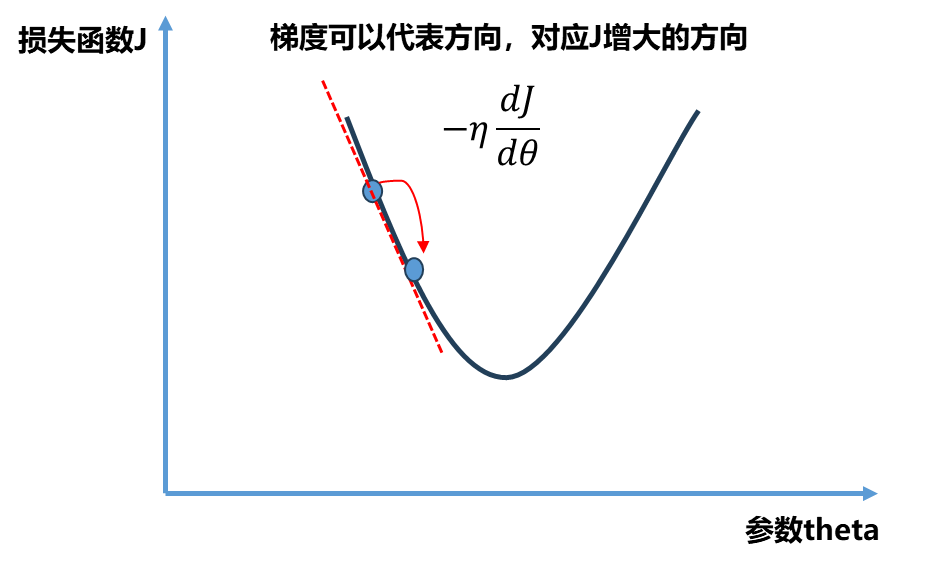
依旧看下面一个二维平面,x x x θ \theta θ y y y
其中η \eta η η \eta η
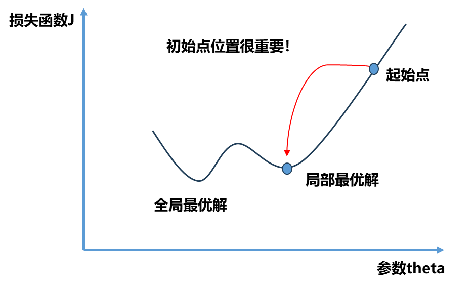
不是所有的函数都有唯一的极值点 ,上面图中二次曲线有唯一的极值点属于简单情况.事实上很多函数是非常复杂的比如下图所示。同时初始点位置也很重要,如果我们起始点在下图右侧就滑入了局部最优解,如果在左侧就滑入了全局最优解,所以我们需要多次随机初始化我们的初始点 ,每次运行比较我们得到的最优解。因此梯度下降法的初始点的位置 也是一个超参数 。
模拟实现梯度下降
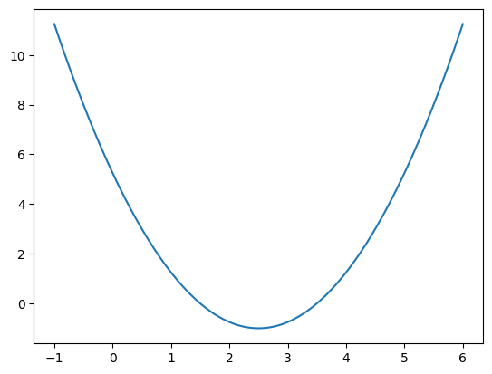
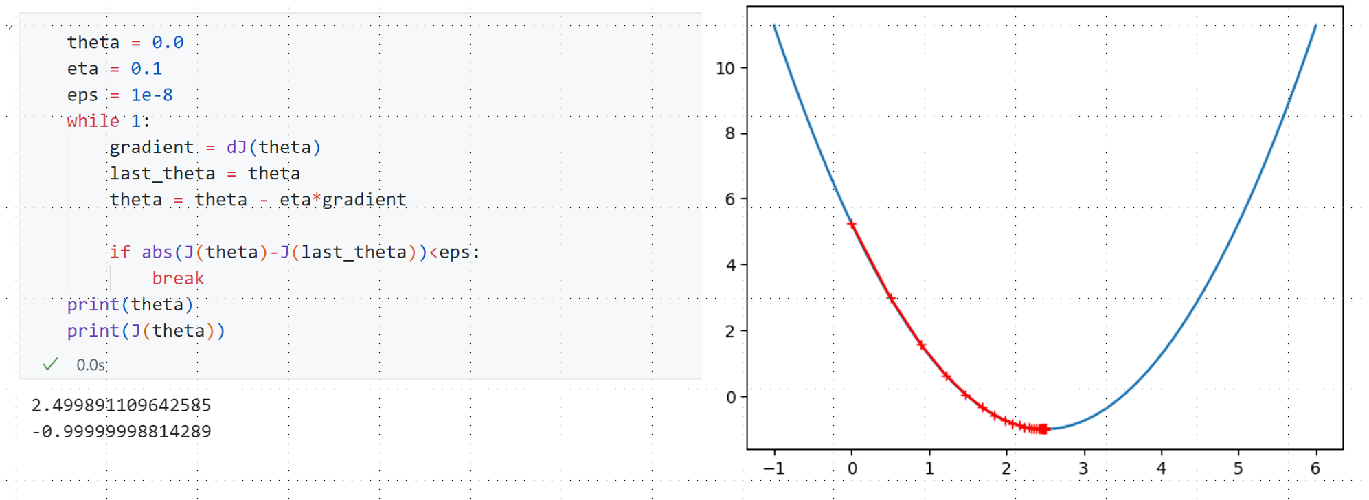
为了可视化方便依旧选用二次函数y = ( x − 2.5 ) 2 − 1 y=(x-2.5)^2-1 y = ( x − 2.5 ) 2 − 1
实现梯度下降法每一次都要计算损失函数对应的梯度,对上述函数求导d J / d θ = 2 ∗ ( θ − 2.5 ) dJ/d\theta = 2*(\theta-2.5) dJ / d θ = 2 ∗ ( θ − 2.5 ) θ \theta θ J = ( θ − 2.5 ) 2 − 1 J=(\theta-2.5)^2-1 J = ( θ − 2.5 ) 2 − 1
1
2
3
4
def dJ (theta ): return 2 *(theta-2.5 ) def J (theta ): return (theta-2.5 )**2 -1
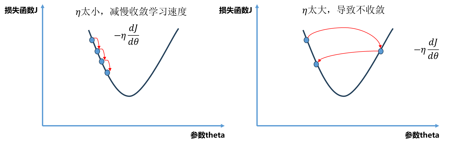
接下来开始梯度下降的过程 :选取0 为初始点,然后开始循环迭代,每一轮循环中首先求得当前点对应的梯度 ,接着θ \theta θ 负方向移动 ,同时这个移动有个步长η \eta η 学习率 ,最后我们要判断当前新的θ \theta θ 编程具体实现时 有可能因为η \eta η θ \theta θ
既然如此,如何判断当前求得的θ \theta θ ?因为每次都是梯度下降,所以理论上每次求到一个新的θ \theta θ θ \theta θ θ \theta θ 精度要求 比如下面设定为ϵ = 1 e − 8 \epsilon=1e-8 ϵ = 1 e − 8
具体实现如下:
最终输出结果θ = 2.4999 , J ( θ ) = − 0.9999 \theta=2.4999,J(\theta)=-0.9999 θ = 2.4999 , J ( θ ) = − 0.9999 J = ( θ − 2.5 ) 2 − 1 J=(\theta-2.5)^2-1 J = ( θ − 2.5 ) 2 − 1 θ \theta θ 46次 查找退出循环。
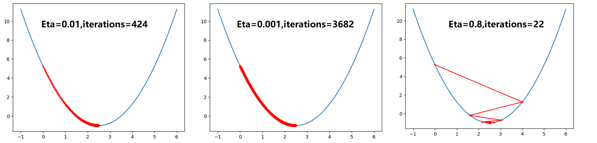
观察不同学习率时η \eta η
η \eta η 0.01 此时明显比取0.1 路径更密,而0.001 则是密集成了一条曲线了。而η \eta η 0.8 可以发现曲线从开始0 点跳到右半端,不过最后还是收敛到最小值点。
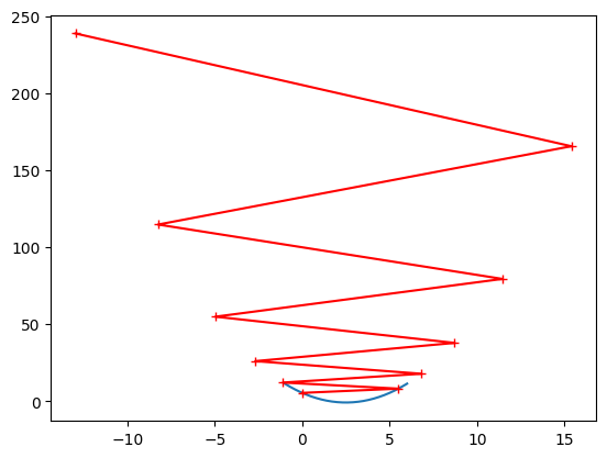
继续取大,当η \eta η OverflowError: (34, ‘Result too large’) .显然是因为此时1.1学习率过大,导致每次损失函数越跳越大,最后知道编译器报出警告。只绘制出前10 次θ \theta θ
多元线性回归中的梯度下降
上面使用一个二次函数曲线模拟了梯度下降的过程,接下来将梯度下降应用到多元线性回归中。前面的博客讲到过多元线性回归的损失函数形式:
J = ∑ i = 1 m ( y ( i ) − y ^ ( i ) ) 2 J=\sum_{i=1}^{m}(y^{(i)}-\hat{y}^{(i)})^2
J = i = 1 ∑ m ( y ( i ) − y ^ ( i ) ) 2
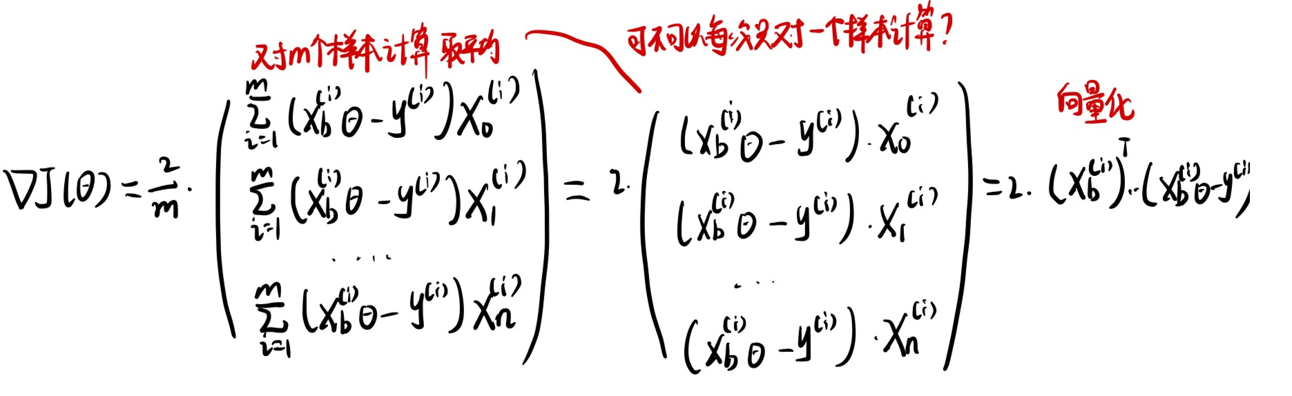
对于多元线性回归来说参数不止一个,n代表样本特征数量:
θ = ( θ 0 , θ 1 , . . . , θ n ) \theta =(\theta_0,\theta_1,...,\theta_n)
θ = ( θ 0 , θ 1 , ... , θ n )
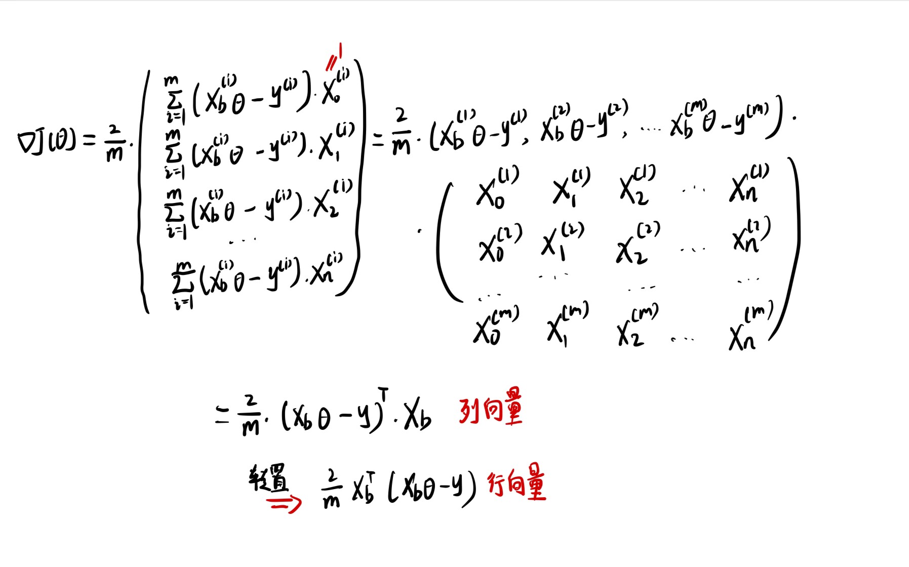
所以我们要将上面二次函数例子中的d J / d θ dJ/d\theta dJ / d θ
∇ J = ( ∂ J ∂ θ 0 , ∂ J ∂ θ 1 , . . . , ∂ J ∂ θ n ) \nabla J=(\frac{\partial J}{\partial\theta_0},\frac{\partial J}{\partial\theta_1},...,\frac{\partial J}{\partial\theta_n})
∇ J = ( ∂ θ 0 ∂ J , ∂ θ 1 ∂ J , ... , ∂ θ n ∂ J )
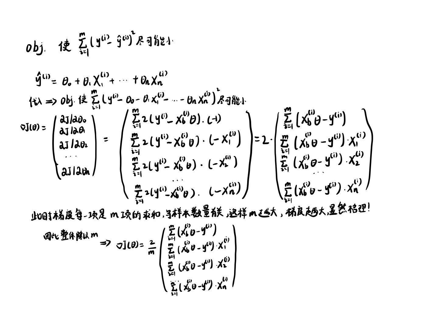
那么接下来详细推导一下线性回归法中的式子是什么样的:
采用上面最后的2 / m 2/m 2/ m
目标 : 使 1 m ∑ i = 1 m ( y ( i ) − y ^ ( i ) ) 2 尽可能小 J ( θ ) = M S E ( y , y ^ ) 目标:使\frac{1}{m}\sum_{i=1}^{m}(y^{(i)}-\hat{y}^{(i)})^2尽可能小\\
J(\theta)=MSE(y,\hat{y})
目标 : 使 m 1 i = 1 ∑ m ( y ( i ) − y ^ ( i ) ) 2 尽可能小 J ( θ ) = MSE ( y , y ^ )
这个推导也说明一个道理:使用梯度下降法来求解一个函数最小值,有时候需要对目标函数进行一些特殊的设计,不见得所有的目标函数都非常的合适。
代码实现 :
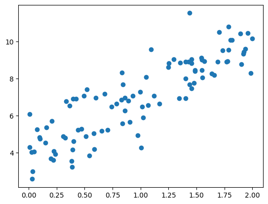
随机生成一组数据满足y = 3 x + 4 y=3x+4 y = 3 x + 4
1
2
3
4
5
6
7
8
9
10
import numpy as npimport matplotlib.pyplot as pltnp.random.seed(666 ) x = 2 *np.random.random(size=100 ) y = x*3. + 4. + np.random.normal(size=100 ) X = x.reshape(-1 ,1 ) plt.scatter(X, y) plt.show()
可视化出来:
接着同上面二次函数中的实现方法一样实现J , d J J,dJ J , dJ
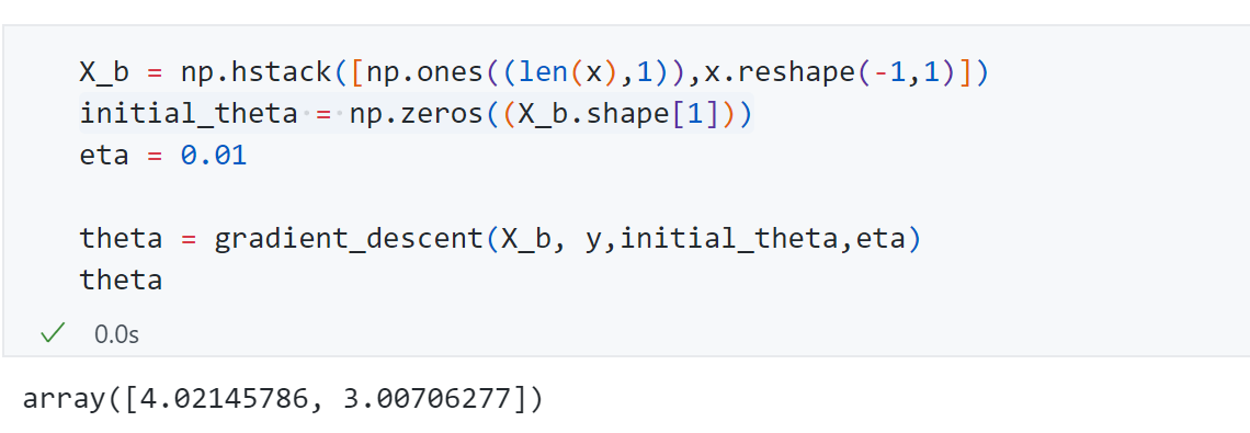
1
2
3
4
5
6
7
8
9
10
11
12
13
14
15
16
17
18
19
20
21
22
23
24
25
26
def J (theta, X_b, y ): try : return np.sum ((y-X_b.dot(theta))**2 )/len (X_b) except : return float ('inf' ) def dJ (theta, X_b, y ): res = np.empty(len (theta)) res[0 ] = np.sum (X_b.dot(theta)-y) for i in range (1 , len (theta)): res[i] = (X_b.dot(theta)-y).dot(X_b[:,i]) return res * 2 /len (X_b) def gradient_descent (X_b, y , initial_theta, eta, n_iters=1e4 , eps=1e-8 ): theta = initial_theta i_iter = 0 while i_iter < n_iters: gradient = dJ(theta, X_b, y) last_theta = theta theta = theta - eta*gradient if abs (J(theta, X_b, y)-J(last_theta,X_b,y)) <eps: break i_iter +=1 return theta
运行得到最终参数 分别为4.02145和3.007符合我们生成的 数据规律。
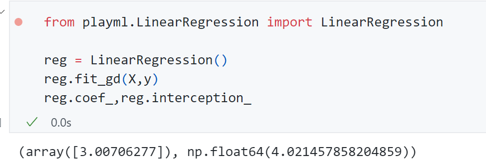
封装方法到之前定义的LinearRegression 类中:
1
2
3
4
5
6
7
8
9
10
11
12
13
14
15
16
17
18
19
20
21
22
23
24
25
26
27
28
29
30
31
32
33
34
35
36
37
38
39
40
def fit_gd (self, X_train, y_train, eta=0.01 , n_iters=1e4 ): assert X_train.shape[0 ] == y_train.shape[0 ],\ "the size of X_train must be equal to the size of y_train" def J (theta, X_b, y ): try : return np.sum ((y-X_b.dot(theta))**2 )/len (X_b) except : return float ('inf' ) def dJ (theta, X_b, y ): res = np.empty(len (theta)) res[0 ] = np.sum (X_b.dot(theta)-y) for i in range (1 , len (theta)): res[i] = (X_b.dot(theta)-y).dot(X_b[:,i]) return res * 2 /len (X_b) def gradient_descent (X_b, y , initial_theta, eta, n_iters=1e4 , eps=1e-8 ): theta = initial_theta i_iter = 0 while i_iter < n_iters: gradient = dJ(theta, X_b, y) last_theta = theta theta = theta - eta*gradient if abs (J(theta, X_b, y)-J(last_theta,X_b,y)) <eps: break i_iter +=1 return theta X_b = np.hstack([np.ones((len (X_train),1 )),X_train]) initial_theta = np.zeros(X_b.shape[1 ]) self ._theta = gradient_descent(X_b, y_train , initial_theta, eta, n_iters=1e4 ) self .interception_ = self ._theta[0 ] self .coef_ = self ._theta[1 :] return self
调用发现结果一致:
向量化
接下来我们依旧尝试对梯度的形式进行向量化来为编程实现上提高效率。
因此接下来可以将d J dJ dJ
1
2
3
4
5
6
7
8
def dJ (theta, X_b, y ): return X_b.T.dot(X_b.dot(theta)-y)*2. /len (y)
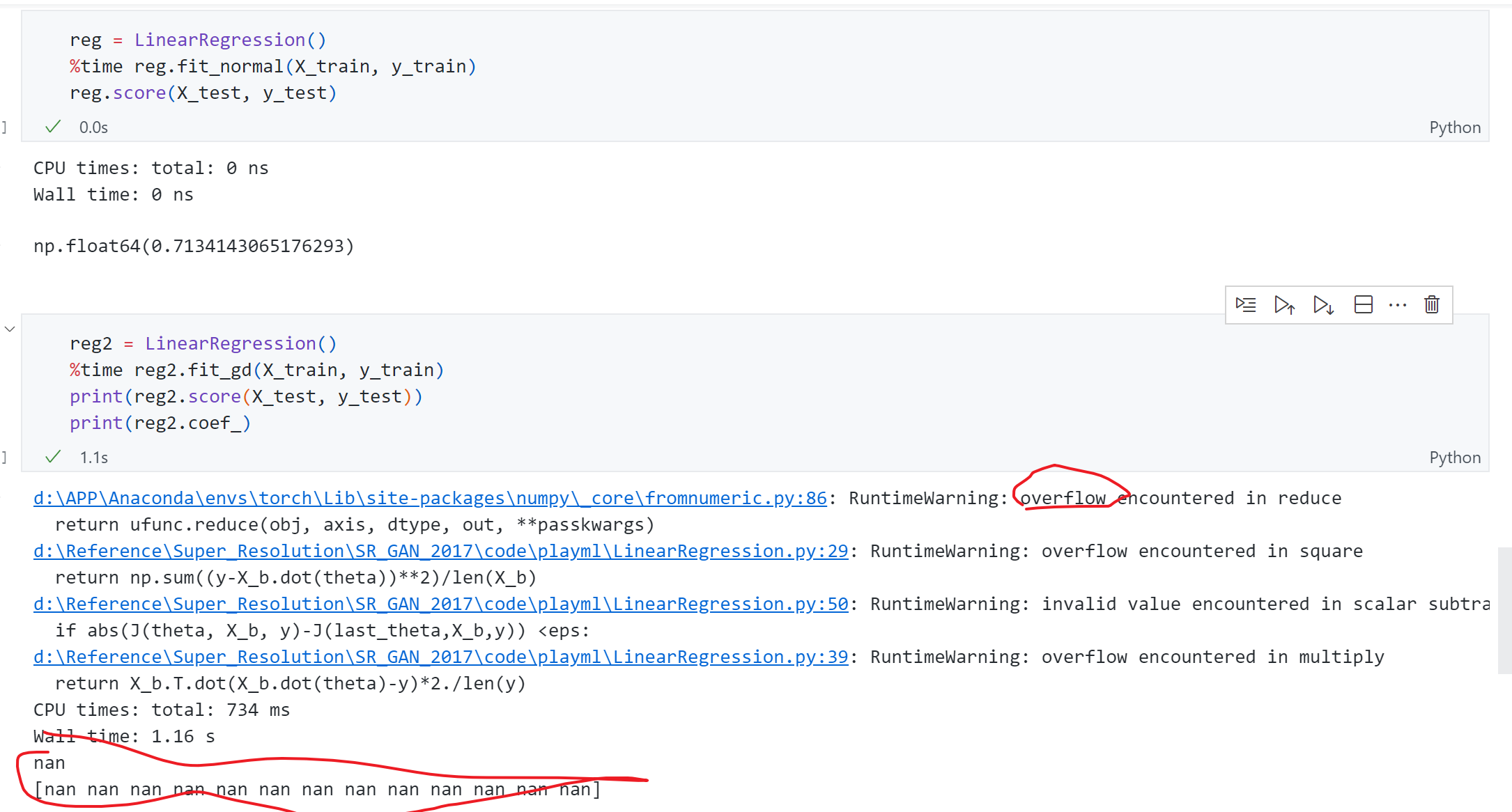
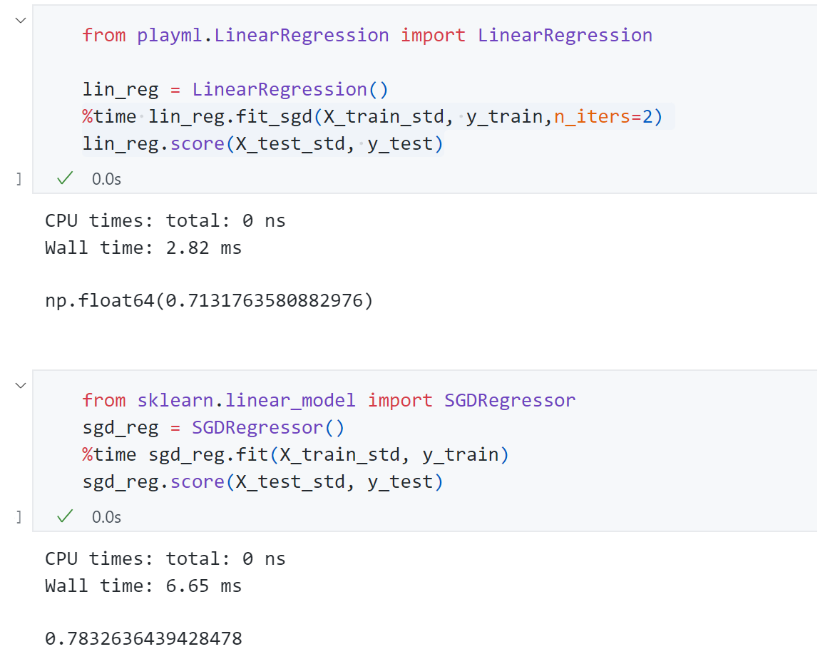
依旧针对Boston housing 数据 进行测试,首先采用正规方程解 的方式 得到score为0.71 ,而采用梯度下降 时出现了overflow报错 ,同时结果全为nan ,这是为什么 ?
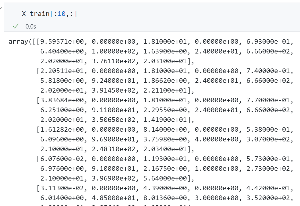
主要原因是现在使用的Boston housing是一个真实数据集,观察一下可以发现每条数据的 各个维度上数据规模差异很大,有些特征是0.多,有些上百多,所以会导致 梯度下降时某些维度的梯度特别大即梯度爆炸。
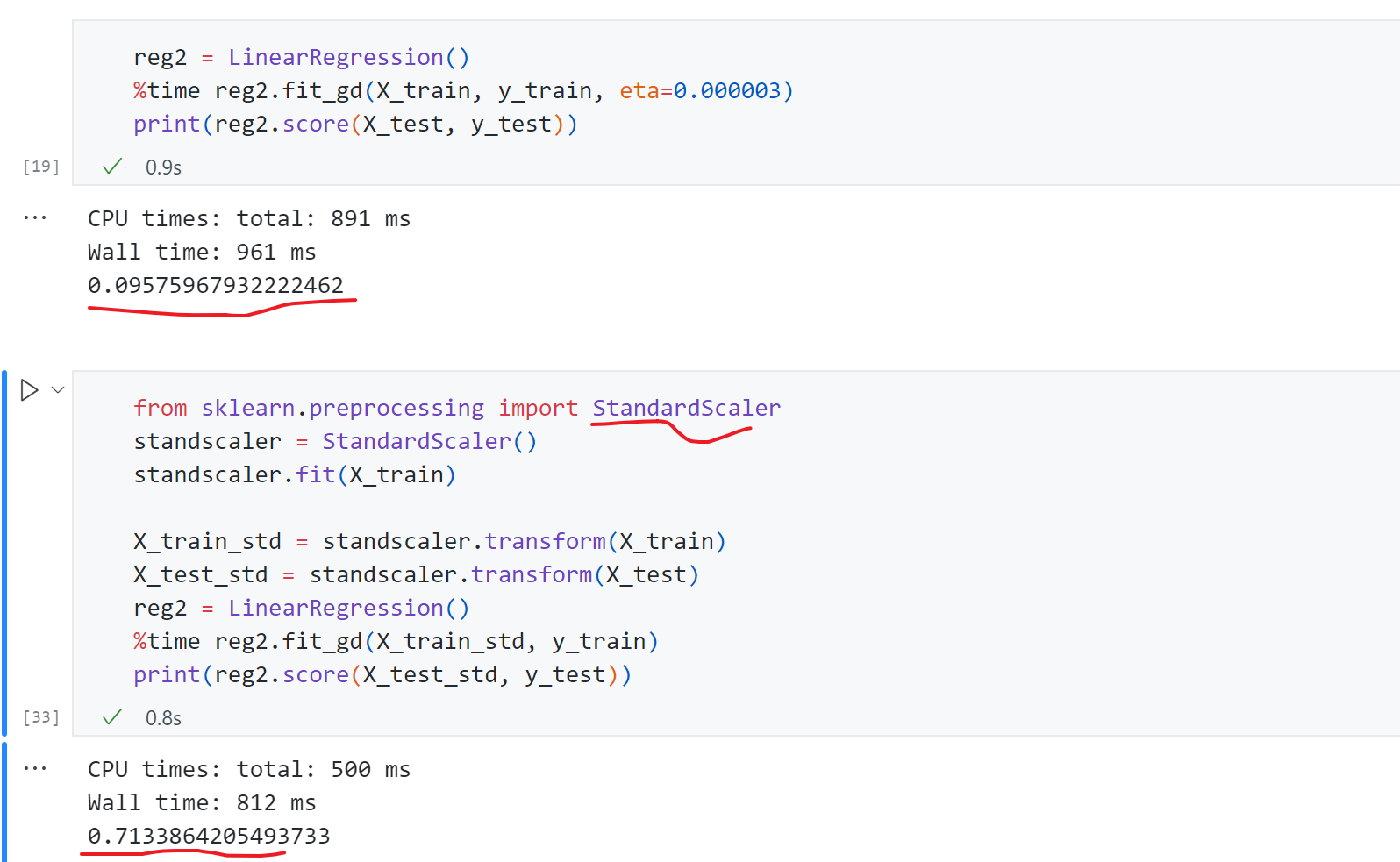
如何验证这一猜想呢?可以先尝试给学习率一个很小的值η = 0.000003 \eta=0.000003 η = 0.000003 θ \theta θ 数据归一化 ,通过数据归一化后我们再使用梯度下降法得到score为0.71,结果恢复了正常。
梯度下降法速度优势
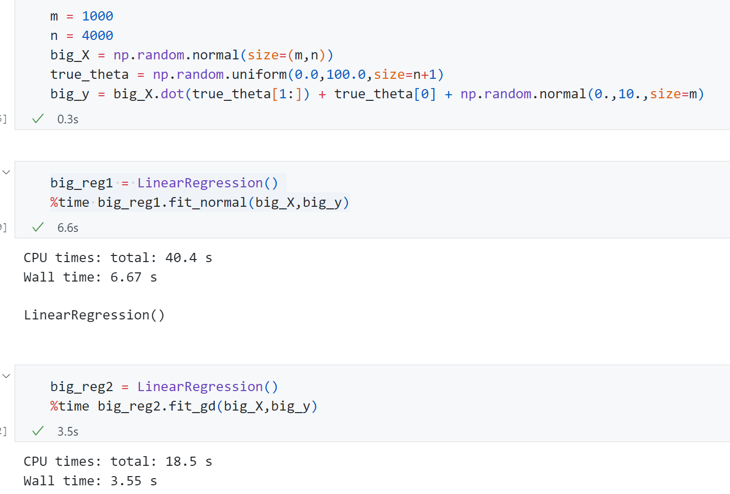
接下来生成随即生成一组样本数量1000,特征数量4000的样本。来比较使用正规方程和梯度下降的速度差异:
可以发现梯度下降法 只用了3.55s ,而正规方程解用了6.67s .如果加大特征数梯度下降法的优势会更加明显。同时可以发现这组数据的样本数量是小于特征量的,我们现在采用的梯度下降法计算梯度时需要每一个样本都参与计算 ,这使得样本量比价大时我们相应计算梯度也比较慢,这也有一种改进的方式 就是-----随机梯度下降法 。
随机梯度下降法
前面推导多元线性回归时用到的梯度下降法每一项都要对所有的m即样本数进行计算,这种梯度下降法也叫做Batch Gradient Descent .这样显然也有一个问题就是如果样本数量m很大,那么计算梯度会非常耗时。‘
尝试将原来m个样本计算梯度变为计算一个样本:
最终得到的式子可以作为我们搜索的方向,没说梯度的方向因为这个式子本身不是损失函数的梯度了。每次都随机取出一个样本i,然后计算这个式子得到一个方向不断搜索迭代,这样思想实现思路就是随机梯度下降法(Stochastic Gradient Descent) .
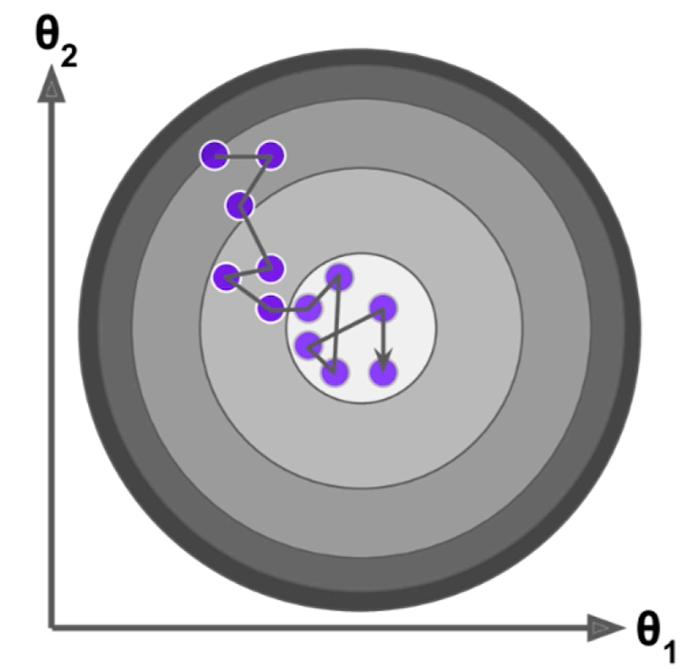
随机梯度下降的搜索过程可能如下面这个图所示,随机梯度下降不能保证每次得到的方向是损失函数减少的方向,更不能保证是减小方向最快的方向。
同时在具体实现的时候,在随机梯度下降法过程中学习率取值非常重要 ,因为随机梯度下降过程如果学习率一直取一个固定值的情况下,很有可能已经来到最小值中心左右位置时但是随机过程不够好同时η \eta η 学习率是逐渐递减 的。
那么可以设置一个函数使得学习率随着循环次数增加越来越小,一个简单的思路是采用 循环次数的倒数:
η = 1 n _ i t e r s \eta=\frac{1}{n\_{iters}}
η = n _ i t ers 1
但这个函数的一个问题是循环次数 比较小的时候η \eta η b b b 模拟退火 的思想。
η = a n _ i t e r s + b \eta=\frac{a}{n\_iters+b}
η = n _ i t ers + b a
编程实现:
1
2
3
4
5
6
7
8
9
import numpy as npimport matplotlib.pyplot as pltm =1000000 x = np.random.normal(size=m) X = x.reshape(-1 ,1 ) X.shape y = 4. *x + 3. + np.random.normal(0 ,3 ,size=m)
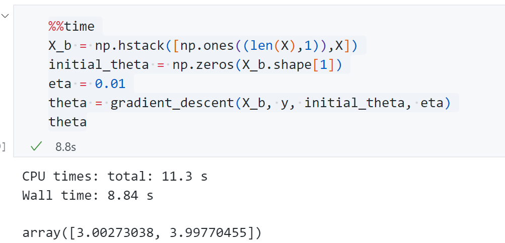
先看一下 采用 Batch Gradient Descent 耗时:
1
2
3
4
5
6
7
8
9
10
11
12
13
14
15
16
17
18
19
20
21
22
23
def J (theta, X_b, y ): try : return np.sum ((y-X_b.dot(theta))**2 )/len (y) except : return float ('inf' ) def dJ (theta, X_b,y ): return X_b.T.dot(X_b.dot(theta)-y)*2. /len (y) def gradient_descent (X_b, y ,initial_theta, eta,n_iters=1e4 ,eps=1e-8 ): theta = initial_theta cur_iter = 0 while cur_iter < n_iters: gradient = dJ(theta,X_b,y) last_theta = theta theta = theta - eta*gradient if (abs (J(theta,X_b,y)-J(last_theta,X_b,y))<eps): break cur_iter+=1 return theta
耗时11.3s,预测的两个系数分别为3.00和3.99,与我们生成给的参数基本一致。
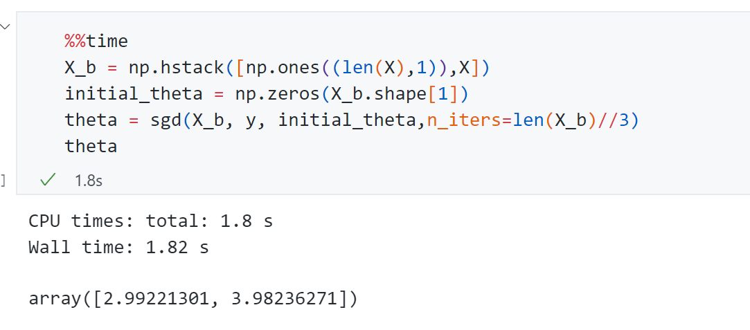
1
2
3
4
5
6
7
8
9
10
11
12
13
14
15
16
17
def dJ_sgd (theta, X_b_i,y_i ): return X_b_i.T.dot(X_b_i.dot(theta)-y_i)*2 def sgd (X_b, y ,initial_theta,n_iters=1e4 ): t0=5 t1=50 def learning_rate (t ): return t0/(t+t1) theta = initial_theta for cur_iter in range (n_iters): rand_i = np.random.randint(len (X_b)) gradient = dJ_sgd(theta,X_b[rand_i],y[rand_i]) theta = theta - learning_rate(cur_iter)*gradient return theta
耗时1.8s,结果2.99和3.98与我们 生成的参数一致,但速度比Batch Gradient Descent快了5-6倍。
同理接下来对SGD方法进行封装:
1
2
3
4
5
6
7
8
9
10
11
12
13
14
15
16
17
18
19
20
21
22
23
24
25
26
27
28
29
30
def fit_sgd (self, X_train, y_train, n_iters=5 , t0=5 , t1=50 ): assert X_train.shape[0 ] == y_train.shape[0 ],\ "the size of X_train must be equal to the size of y_train" def dJ_sgd (theta, X_b_i,y_i ): return X_b_i.T.dot(X_b_i.dot(theta)-y_i)*2 def sgd (X_b, y ,initial_theta,n_iters=1e4 ,t0=5 ,t1=50 ): def learning_rate (t ): return t0/(t+t1) theta = initial_theta m = len (X_b) for cur_iter in range (n_iters): indexes = np.random.permutation(m) X_b_new = X_b[indexes] y_new = y[indexes] for i in range (m): gradient = dJ_sgd(theta,X_b_new[i],y_new[i]) theta = theta - learning_rate(cur_iter*m+i)*gradient return theta X_b = np.hstack([np.ones((len (X_train),1 )),X_train]) initial_theta = np.zeros(X_b.shape[1 ]) self ._theta = sgd(X_b, y_train , initial_theta,n_iters,t0,t1) self .interception_ = self ._theta[0 ] self .coef_ = self ._theta[1 :] return self
依旧应用到 Boston Housing数据上:
可以发现scikit-learn的效果比我们实现的效果要好。
梯度的调试(*)
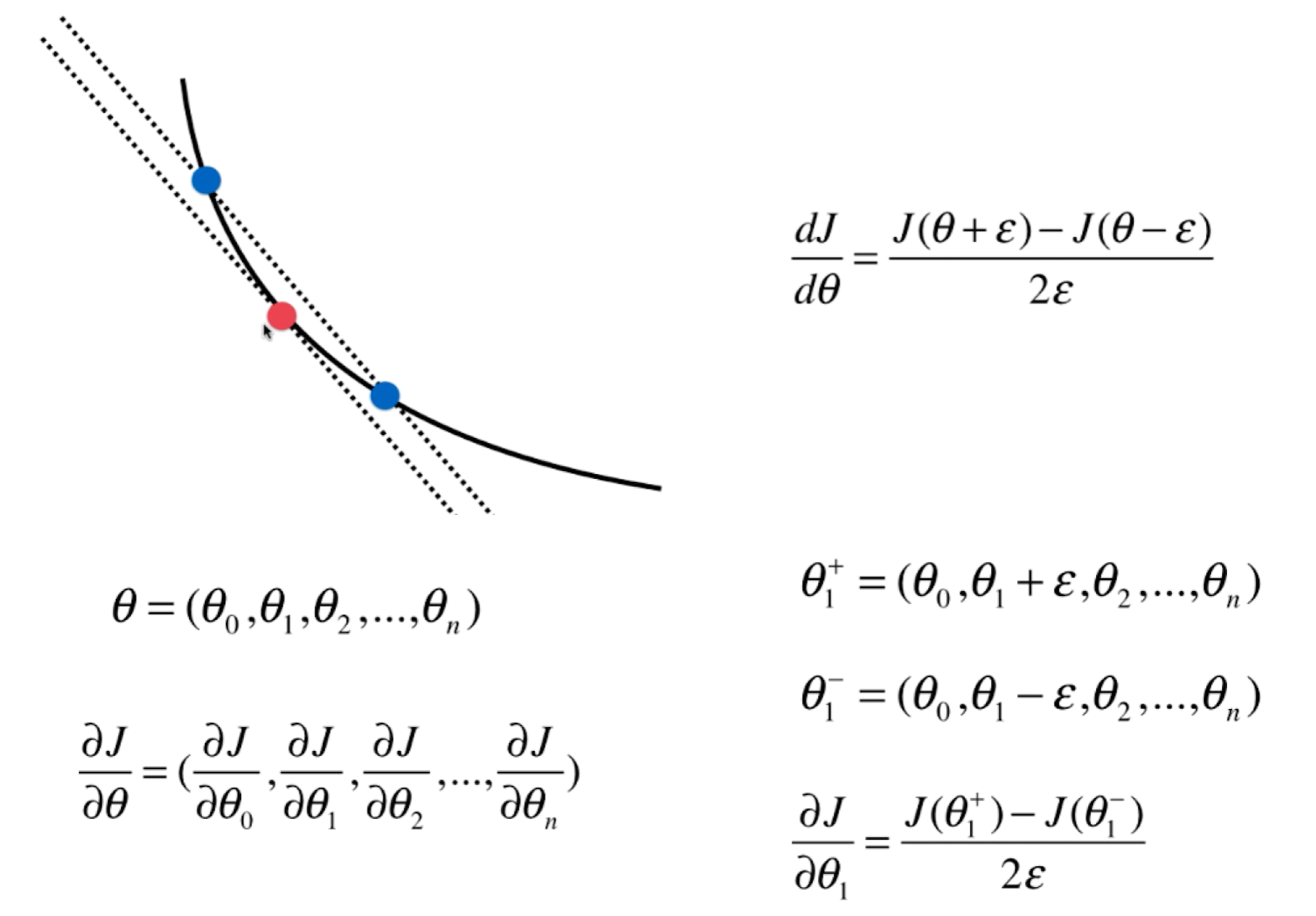
使用梯度下降法很重要的一个点是求出损失函数在对应θ \theta θ
对于一个点的梯度我们可以导数定义出发,通过在红点左右分别取一蓝点,当这个间距越小,此时这个斜率越接近红点的导数。同样对于多维度对每个维度用这种方式求解即可。
代码实现:
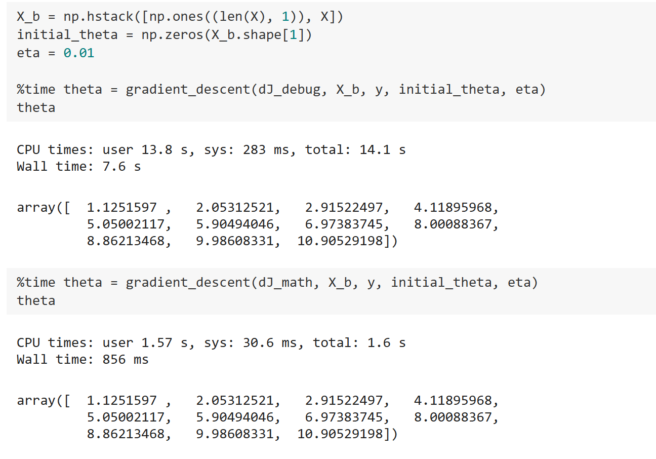
1
2
3
4
5
6
7
8
9
10
11
12
13
14
15
16
17
18
19
20
21
22
23
24
25
26
27
28
29
30
31
32
33
34
35
36
37
38
39
40
import numpy as npimport matplotlib.pyplot as pltnp.random.seed(666 ) X = np.random.random(size=(1000 , 10 )) true_theta = np.arange(1 , 12 , dtype=float ) X_b = np.hstack([np.ones((len (X), 1 )), X]) y = X_b.dot(true_theta) + np.random.normal(size=1000 ) def J (theta, X_b, y ): try : return np.sum ((y - X_b.dot(theta))**2 ) / len (X_b) except : return float ('inf' ) def dJ_math (theta, X_b, y ): return X_b.T.dot(X_b.dot(theta) - y) * 2. / len (y) def dJ_debug (theta, X_b, y, epsilon=0.01 ): res = np.empty(len (theta)) for i in range (len (theta)): theta_1 = theta.copy() theta_1[i] += epsilon theta_2 = theta.copy() theta_2[i] -= epsilon res[i] = (J(theta_1, X_b, y) - J(theta_2, X_b, y)) / (2 * epsilon) return res def gradient_descent (dJ, X_b, y, initial_theta, eta, n_iters = 1e4 , epsilon=1e-8 ): theta = initial_theta cur_iter = 0 while cur_iter < n_iters: gradient = dJ(theta, X_b, y) last_theta = theta theta = theta - eta * gradient if (abs (J(theta, X_b, y) - J(last_theta, X_b, y)) < epsilon): break cur_iter += 1 return theta
观察结果:
可以发现使用d J d e b u g dJ_{debug} d J d e b ug d J d e b u g dJ_{debug} d J d e b ug d J d e b u g dJ_{debug} d J d e b ug d J d e b u g dJ_{debug} d J d e b ug d J m a t h dJ_{math} d J ma t h 所以d J d e b u g dJ_{debug} d J d e b ug 。
一些思考总结
前面主要说了两种梯度下降法:
批量梯度下降法 Batch Gradient Descent :对所有的样本求解,速度慢,但是稳定,一定可以向损失函数下降最快方向前进。
随机梯度下降法 Stochastic Gradient Descent :每次只对一个样本求解,快,但是不稳定,甚至可能反方向前进。
综合这两种梯度下降法就有了小批量梯度下降法Mini-Batch Gradient Descent ,每次看k个样本,兼顾两种方法。
同时梯度下降法不是一个机器学习算法 ,是一种基于搜索的最优化方法 ,可以最小化一个损失函数或者梯度上升法最大化一个效用函数。