Logistic Regression
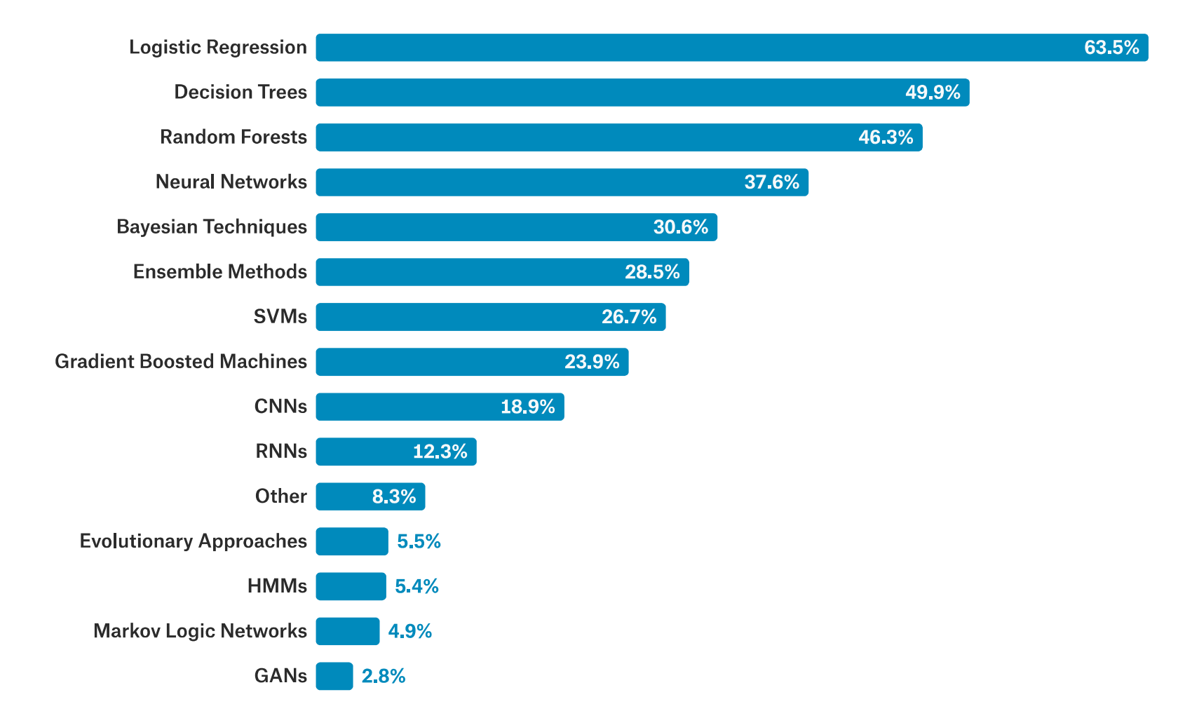
kaggle 在2017 年发布了一篇名为"The State of Data Science and Machine Learning "的报告,报告里面有这样一个问题:
1
2
3
4
What data science methods are used at work? Logistic regression is the most commonly reported data science method used at work for all industries except Military and Security where Neural Networks are used slightly more frequently.
大意就是逻辑回归 是各行业中工作中最常使用的数据科学方法,除了在军事和安全领域中,因为军事安全领域神经网络的使用频率略高一些。同时里面有这样一张图:
可以发现2017年 之前逻辑回归、决策树、随机森林 是当时使用率的前三名 ,相比而言CNN、RNN 等深度学习方法排名相对靠后 。逻辑回归算法思路比较简单,使用率排名第一,可见其非常有用。
什么是逻辑回归?
逻辑回归(Logistic Regression)从名字上看是一个回归算法,但其主要用来 解决分类问题 的。那么回归算法怎么解决分类问题呢?逻辑回归主要原理是将样本特征和样本发生的概率 联系起来,即预测样本发生的概率是多少,概率是一个数,所以可以当作一个回归问题。
机器学习算法本质是求出一个函数f f f x x x y ^ \hat{y} y ^
y ^ = f ( x ) \hat{y}=f(x)
y ^ = f ( x )
对于之前的线性回归、多线性回归等这个y ^ \hat{y} y ^ 概率值 :
p ^ = f ( x ) y ^ = { 1 , p ^ ≥ 0.5 0 , p ^ < 0.5 \hat{p}=f(x)\\
\hat{y} =
\begin{cases}
1, & \hat{p} \ge 0.5 \\
0, & \hat{p} < 0.5
\end{cases}
p ^ = f ( x ) y ^ = { 1 , 0 , p ^ ≥ 0.5 p ^ < 0.5
根据概率值的大小我们进而可以进行分类,比如上面p ^ ≥ 0.5 \hat{p} \ge0.5 p ^ ≥ 0.5 p ^ < 0.5 \hat{p} <0.5 p ^ < 0.5
逻辑回归既可以看做是回归算法,也可以看做是分类算法。通常作为分类算法用,只可以解决二分类问题。而KNN算法天生可以解决多分类问题,逻辑回归需要一些其他技巧改进才可以解决多分类问题。
那么逻辑回归通过什么样的方式来得到一个事件的概率值?线性回归中:
y ^ = θ T . x b 值域 ( − i n f , + i n f ) 概率的值域 [ 0 , 1 ] \hat{y}=\theta^T.x_b \quad 值域(-inf,+inf)\\
概率的值域[0,1]
y ^ = θ T . x b 值域 ( − in f , + in f ) 概率的值域 [ 0 , 1 ]
如果直接用y ^ \hat {y} y ^ σ \sigma σ
p ^ = σ ( θ T . x b ) \hat{p}=\sigma(\theta^T.x_b)
p ^ = σ ( θ T . x b )
此时值域就变为了[0,1]之间,但这个σ \sigma σ
σ \sigma σ Sigmoid 函数,表达式:
σ ( t ) = 1 1 + e − t \sigma(t)=\frac{1}{1+e^{-t}}
σ ( t ) = 1 + e − t 1
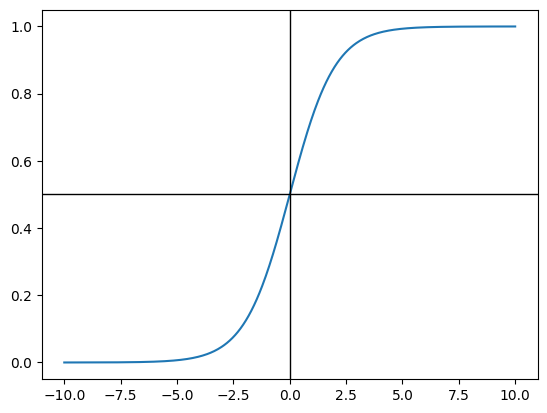
1
2
3
4
5
6
7
8
9
10
11
12
13
import numpy as npimport matplotlib.pyplot as pltdef sigmoid (t ): return 1 / (1 + np.exp(-t)) x = np.linspace(-10 , 10 , 500 ) y = sigmoid(x) plt.plot(x, y) plt.axhline(0.5 , color='black' , linewidth=1 ) plt.axvline(0 , color='black' , linewidth=1 ) plt.show()
可以发现Sigmoid函数值域就在[0,1]之间,当t > 0 t>0 t > 0 p > 0.5 p>0.5 p > 0.5 t < 0 t<0 t < 0 p < 0.5 p<0.5 p < 0.5 t = 0 t=0 t = 0 p = 0.5 p=0.5 p = 0.5
所以整体上逻辑回归的表达式:
p ^ = σ ( θ T . x b ) = 1 1 + e − θ T . x b y ^ = { 1 , p ^ ≥ 0.5 0 , p ^ ≤ 0.5 \hat{p}=\sigma(\theta^T.x_b)=\frac{1}{1+e^{-\theta^T.x_b}}\\
\hat{y}=
\begin{cases}
1, & \hat{p} \ge 0.5\\
0, & \hat{p} \le 0.5
\end{cases}
p ^ = σ ( θ T . x b ) = 1 + e − θ T . x b 1 y ^ = { 1 , 0 , p ^ ≥ 0.5 p ^ ≤ 0.5
那么剩下的问题就是:对于给定的样本数据集X,y,我们如何找到参数theta ,使得用这样的方式可以最大程度获得样本X对应的分类输出y?
逻辑回归的损失函数
回想线性回归中是通过y − y ^ y-\hat{y} y − y ^ MSE 作为损失函数,然后找到让损失函数最小的θ \theta θ 损失函数该如何定义 ?
首先逻辑回归跟前面线性回归最大的一个区别是逻辑回归解决的是分类问题 ,我们要根据估计出来的p ^ \hat{p} p ^ y ^ \hat{y} y ^
c o s t = { 如果 y = 1 , p 越小 , c o s t 越大 如果 y = 0 , p 越大 , c o s t 越大 ↓ c o s t = { − l o g ( p ^ ) i f y = 1 − l o g ( 1 − p ^ ) i f y = 0 cost=
\begin{cases}
如果y=1,p越小,cost越大\\
如果y=0,p越大,cost越大\\
\end{cases}\\
\downarrow\\
cost=
\begin{cases}
-log(\hat{p})\quad if \quad y=1 \\
-log(1-\hat{p})\quad if \quad y=0\\
\end{cases}\\
cos t = { 如果 y = 1 , p 越小 , cos t 越大 如果 y = 0 , p 越大 , cos t 越大 ↓ cos t = { − l o g ( p ^ ) i f y = 1 − l o g ( 1 − p ^ ) i f y = 0
如何理解呢?这里的y y y y = 1 y=1 y = 1 p p p y ^ \hat{y} y ^ y = 0 y=0 y = 0 p p p y ^ \hat{y} y ^
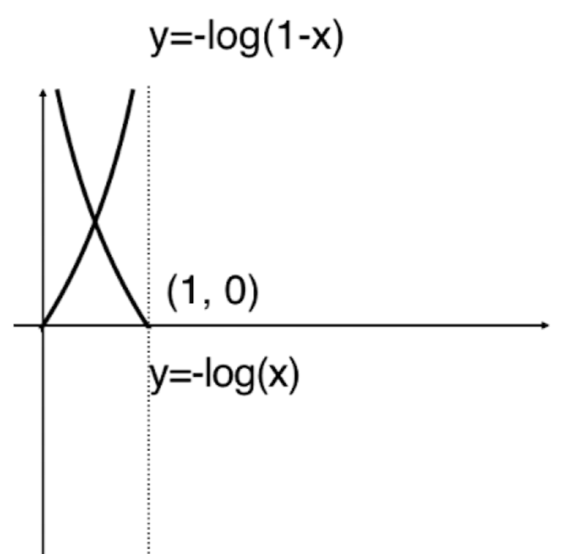
绘制出两个函数图像:
此时无论y = 1 y=1 y = 1 y = 0 y=0 y = 0 y = − l o g ( x ) y=-log(x) y = − l o g ( x ) x x x y = − l o g ( 1 − x ) y=-log(1-x) y = − l o g ( 1 − x )
但此时的惩罚函数整体是一个分类函数,需要依据y y y
c o s t = − y l o g ( p ^ ) − ( 1 − y ) l o g ( 1 − p ^ ) cost=-ylog(\hat{p})-(1-y)log(1-\hat{p})
cos t = − y l o g ( p ^ ) − ( 1 − y ) l o g ( 1 − p ^ )
显然当y = 1 y=1 y = 1 c o s t = − y l o g ( p ^ ) cost=-ylog(\hat p) cos t = − y l o g ( p ^ ) y = 0 y=0 y = 0 c o s t = − ( 1 − y ) l o g ( 1 − p ^ ) cost=-(1-y)log(1-\hat{p}) cos t = − ( 1 − y ) l o g ( 1 − p ^ )
上面是一个样本的情况,对于m个样本 就是:
J ( θ ) = − 1 m ∑ i = 1 m y ( i ) l o g ( p ^ ( i ) ) + ( 1 − y ( i ) ) l o g ( 1 − p ^ ( i ) ) p ^ ( i ) = σ ( X b ( i ) θ ) = 1 1 + e − X b ( i ) θ J(\theta)=-\frac{1}{m}\sum_{i=1}^{m}y^{(i)}log(\hat{p}^{(i)})+(1-y^{(i)})log(1-\hat{p}^{(i)})\\
\hat{p}^{(i)}=\sigma(X^{(i)}_b\theta)=\frac{1}{1+e^{-X_b^{(i)}\theta}}
J ( θ ) = − m 1 i = 1 ∑ m y ( i ) l o g ( p ^ ( i ) ) + ( 1 − y ( i ) ) l o g ( 1 − p ^ ( i ) ) p ^ ( i ) = σ ( X b ( i ) θ ) = 1 + e − X b ( i ) θ 1
到此,我们的目标就是找到一组θ \theta θ J ( θ ) J(\theta) J ( θ ) J ( θ ) J(\theta) J ( θ ) 只能使用梯度下降法求解 。
逻辑回归损失函数梯度推导
观察到J ( θ ) J(\theta) J ( θ ) σ \sigma σ σ \sigma σ
σ ( t ) = 1 1 + e − t = ( 1 + e − t ) − 1 σ ( t ) , = − ( 1 + e − t ) − 2 . ( − e − t ) = ( 1 + e − t ) − 2 . e − t \sigma(t)=\frac{1}{1+e^{-t}}=(1+e^{-t})^{-1}\\
\sigma(t)^{,}=-(1+e^{-t})^{-2}.(-e^{-t})=(1+e^{-t})^{-2}.e^{-t}
σ ( t ) = 1 + e − t 1 = ( 1 + e − t ) − 1 σ ( t ) , = − ( 1 + e − t ) − 2 . ( − e − t ) = ( 1 + e − t ) − 2 . e − t
在此基础上对l o g σ ( t ) log\sigma(t) l o g σ ( t )
( l o g σ ( t ) ) , = σ ( t ) , σ ( t ) = 1 σ ( t ) . ( 1 + e − t ) − 2 . e − t = 1 ( 1 + e − t ) − 1 . ( 1 + e − t ) − 2 . e − t = ( 1 + e − t ) − 1 . e − t = e − t 1 + e − t = 1 − 1 1 + e − t = 1 − σ ( t ) (log\sigma(t))^,=\frac{\sigma(t)^,}{\sigma(t)}=\frac{1}{\sigma(t)}.(1+e^{-t})^{-2}.e^{-t}\\
=\frac{1}{(1+e^{-t})^{-1}}.(1+e^{-t})^{-2}.e^{-t}\\
=(1+e^{-t})^{-1}.e^{-t}\\
=\frac{e^{-t}}{1+e^{-t}}=1-\frac{1}{1+e^{-t}}\\
=1-\sigma(t)
( l o g σ ( t ) ) , = σ ( t ) σ ( t ) , = σ ( t ) 1 . ( 1 + e − t ) − 2 . e − t = ( 1 + e − t ) − 1 1 . ( 1 + e − t ) − 2 . e − t = ( 1 + e − t ) − 1 . e − t = 1 + e − t e − t = 1 − 1 + e − t 1 = 1 − σ ( t )
同理看一下l o g ( 1 − σ ( t ) ) log(1-\sigma(t)) l o g ( 1 − σ ( t ))
( l o g ( 1 − σ ( t ) ) ) , = − σ ( t ) , 1 − σ ( t ) = − ( 1 + e − t ) − 2 . e − t 1 − σ ( t ) = − ( 1 + e − t ) − 2 . e − t 1 − ( 1 + e − t ) − 1 = − ( 1 + e − t ) − 1 . e − t 1 + e − t − 1 = − ( 1 + e − t ) − 1 = − σ ( t ) (log(1-\sigma(t)))^,=\frac{-\sigma(t)^,}{1-\sigma(t)}=\frac{-(1+e^{-t})^{-2}.e^{-t}}{1-\sigma(t)}\\
=\frac{-(1+e^{-t})^{-2}.e^{-t}}{1-(1+e^{-t})^{-1}}\\
=\frac{-(1+e^{-t})^{-1}.e^{-t}}{1+e^{-t}-1}\\
=-(1+e^{-t})^{-1}\\
=-\sigma(t)
( l o g ( 1 − σ ( t )) ) , = 1 − σ ( t ) − σ ( t ) , = 1 − σ ( t ) − ( 1 + e − t ) − 2 . e − t = 1 − ( 1 + e − t ) − 1 − ( 1 + e − t ) − 2 . e − t = 1 + e − t − 1 − ( 1 + e − t ) − 1 . e − t = − ( 1 + e − t ) − 1 = − σ ( t )
因此可得到J ( θ ) J(\theta) J ( θ ) θ j \theta_j θ j
J ( θ ) = − 1 m ∑ i = 1 m y ( i ) l o g ( p ^ ( i ) ) + ( 1 − y ( i ) ) l o g ( 1 − p ^ ( i ) ) d ( y ( i ) l o g ( σ ( X b ( i ) θ ) ) ) d θ j = y ( i ) ( 1 − σ ( X b ( i ) θ ) ) . X j ( i ) d ( ( 1 − y ( i ) ) l o g ( 1 − σ ( X b ( i ) θ ) ) ) d θ j = ( 1 − y ( i ) ) ( − σ ( X b ( i ) θ ) ) . X j ( i ) J ( θ ) θ j = − 1 m ∑ i = 1 m ( y ( i ) ( 1 − σ ( X b ( i ) θ ) ) . X j ( i ) + ( 1 − y ( i ) ) ( − σ ( X b ( i ) θ ) ) . X j ( i ) ) = − 1 m ∑ i = 1 m ( y ( i ) . X j ( i ) − y ( i ) σ ( X b ( i ) θ ) . X j ( i ) − σ ( X b ( i ) θ ) . X j ( i ) + y ( i ) σ ( X b ( i ) θ ) . X j ( i ) ) = − 1 m ∑ i = 1 m ( y ( i ) . X j ( i ) − σ ( X b ( i ) θ ) . X j ( i ) ) = − 1 m ∑ i = 1 m ( y ( i ) − σ ( X b ( i ) θ ) ) . X j ( i ) = 1 m ∑ i = 1 m ( σ ( X b ( i ) θ ) − y ( i ) ) . X j ( i ) = 1 m ∑ i = 1 m ( y ^ ( i ) − y ( i ) ) . X j ( i ) J(\theta)=-\frac{1}{m}\sum_{i=1}^{m}y^{(i)}log(\hat{p}^{(i)})+(1-y^{(i)})log(1-\hat{p}^{(i)})\\
\frac{d(y^{(i)}log(\sigma(X_b^{(i)}\theta)))}{d\theta_j}=y^{(i)}(1-\sigma(X_b^{(i)}\theta)).X_j^{(i)}\\
\frac{d((1-y^{(i)})log(1-\sigma(X_b^{(i)}\theta)))}{d\theta_j}=(1-y^{(i)})(-\sigma(X_b^{(i)}\theta)).X_j^{(i)}\\
\frac{J(\theta)}{\theta_j}=-\frac{1}{m}\sum_{i=1}^{m}(y^{(i)}(1-\sigma(X_b^{(i)}\theta)).X_j^{(i)}+(1-y^{(i)})(-\sigma(X_b^{(i)}\theta)).X_j^{(i)})\\=-\frac{1}{m}\sum_{i=1}^{m}(y^{(i)}.X_j^{(i)}-y^{(i)}\sigma(X_b^{(i)}\theta).X_j^{(i)}-\sigma(X_b^{(i)}\theta).X_j^{(i)}+y^{(i)}\sigma(X_b^{(i)}\theta).X_j^{(i)})\\
=-\frac{1}{m}\sum_{i=1}^{m}(y^{(i)}.X_j^{(i)}-\sigma(X_b^{(i)}\theta).X_j^{(i)})\\
=-\frac{1}{m}\sum_{i=1}^{m}(y^{(i)}-\sigma(X_b^{(i)}\theta)).X_j^{(i)}\\
=\frac{1}{m}\sum_{i=1}^{m}(\sigma(X_b^{(i)}\theta)-y^{(i)}).X_j^{(i)}\\
=\frac{1}{m}\sum_{i=1}^{m}(\hat{y}^{(i)}-y^{(i)}).X_j^{(i)}
J ( θ ) = − m 1 i = 1 ∑ m y ( i ) l o g ( p ^ ( i ) ) + ( 1 − y ( i ) ) l o g ( 1 − p ^ ( i ) ) d θ j d ( y ( i ) l o g ( σ ( X b ( i ) θ ))) = y ( i ) ( 1 − σ ( X b ( i ) θ )) . X j ( i ) d θ j d (( 1 − y ( i ) ) l o g ( 1 − σ ( X b ( i ) θ ))) = ( 1 − y ( i ) ) ( − σ ( X b ( i ) θ )) . X j ( i ) θ j J ( θ ) = − m 1 i = 1 ∑ m ( y ( i ) ( 1 − σ ( X b ( i ) θ )) . X j ( i ) + ( 1 − y ( i ) ) ( − σ ( X b ( i ) θ )) . X j ( i ) ) = − m 1 i = 1 ∑ m ( y ( i ) . X j ( i ) − y ( i ) σ ( X b ( i ) θ ) . X j ( i ) − σ ( X b ( i ) θ ) . X j ( i ) + y ( i ) σ ( X b ( i ) θ ) . X j ( i ) ) = − m 1 i = 1 ∑ m ( y ( i ) . X j ( i ) − σ ( X b ( i ) θ ) . X j ( i ) ) = − m 1 i = 1 ∑ m ( y ( i ) − σ ( X b ( i ) θ )) . X j ( i ) = m 1 i = 1 ∑ m ( σ ( X b ( i ) θ ) − y ( i ) ) . X j ( i ) = m 1 i = 1 ∑ m ( y ^ ( i ) − y ( i ) ) . X j ( i )
进而逻辑回归损失函数梯度 表达式:
▽ J ( θ ) = ( ∂ J ∂ w 0 ∂ J ∂ w 1 . . . ∂ J ∂ w n ) = 1 m ( ∑ i = 1 m ( σ ( X b ( i ) θ ) − y ( i ) ) .1 ∑ i = 1 m ( σ ( X b ( i ) θ ) − y ( i ) ) . X 1 ( i ) . . . ∑ i = 1 m ( σ ( X b ( i ) θ ) − y ( i ) ) . X n ( i ) ) = 1 m ( ∑ i = 1 m ( y ^ ( i ) − y ( i ) ) .1 ∑ i = 1 m ( y ^ ( i ) − y ( i ) ) . X 1 ( i ) . . . ∑ i = 1 m ( y ^ ( i ) − y ( i ) ) . X n ( i ) ) \triangledown J(\theta)=\begin{pmatrix}
\frac{\partial J}{\partial w_0} \\
\frac{\partial J}{\partial w_1} \\
...\\
\frac{\partial J}{\partial w_n}
\end{pmatrix}
= \frac{1}{m}
\begin{pmatrix}
\sum_{i=1}^{m}(\sigma(X_b^{(i)}\theta)-y^{(i)}).1 \\
\sum_{i=1}^{m}(\sigma(X_b^{(i)}\theta)-y^{(i)}).X_1^{(i)} \\
...\\
\sum_{i=1}^{m}(\sigma(X_b^{(i)}\theta)-y^{(i)}).X_n^{(i)}
\end {pmatrix}\\
= \frac{1}{m}
\begin{pmatrix}
\sum_{i=1}^{m}(\hat{y}^{(i)}-y^{(i)}).1 \\
\sum_{i=1}^{m}(\hat{y}^{(i)}-y^{(i)}).X_1^{(i)} \\
...\\
\sum_{i=1}^{m}(\hat{y}^{(i)}-y^{(i)}).X_n^{(i)}
\end {pmatrix}\\
▽ J ( θ ) = ∂ w 0 ∂ J ∂ w 1 ∂ J ... ∂ w n ∂ J = m 1 ∑ i = 1 m ( σ ( X b ( i ) θ ) − y ( i ) ) .1 ∑ i = 1 m ( σ ( X b ( i ) θ ) − y ( i ) ) . X 1 ( i ) ... ∑ i = 1 m ( σ ( X b ( i ) θ ) − y ( i ) ) . X n ( i ) = m 1 ∑ i = 1 m ( y ^ ( i ) − y ( i ) ) .1 ∑ i = 1 m ( y ^ ( i ) − y ( i ) ) . X 1 ( i ) ... ∑ i = 1 m ( y ^ ( i ) − y ( i ) ) . X n ( i )
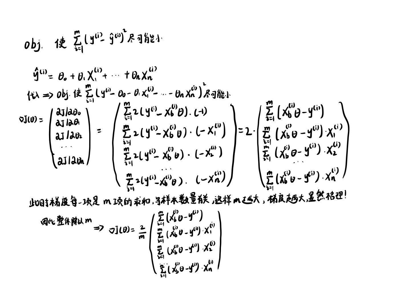
在这里顺便回想一下线性回归的梯度表达式 :
可以发现两者区别在于线性回归是X b ( i ) θ X_b^{(i)}\theta X b ( i ) θ σ ( X b i θ ) \sigma(X_b^{i}\theta) σ ( X b i θ ) y ^ ( i ) − y ( i ) \hat{y}^{(i)}-y^{(i)} y ^ ( i ) − y ( i )
向量化
对上面推导出的逻辑回归梯度表达式 进行向量化 :
▽ J ( θ ) = = 1 m ( ∑ i = 1 m ( y ^ ( i ) − y ( i ) ) .1 ∑ i = 1 m ( y ^ ( i ) − y ( i ) ) . X 1 ( i ) ∑ i = 1 m ( y ^ ( i ) − y ( i ) ) . X 2 ( i ) . . . ∑ i = 1 m ( y ^ ( i ) − y ( i ) ) . X n ( i ) ) = 1 m . X b T . ( σ ( X b θ ) − y ) \triangledown J(\theta)=
= \frac{1}{m}
\begin{pmatrix}
\sum_{i=1}^{m}(\hat{y}^{(i)}-y^{(i)}).1 \\
\sum_{i=1}^{m}(\hat{y}^{(i)}-y^{(i)}).X_1^{(i)} \\
\sum_{i=1}^{m}(\hat{y}^{(i)}-y^{(i)}).X_2^{(i)} \\
...\\
\sum_{i=1}^{m}(\hat{y}^{(i)}-y^{(i)}).X_n^{(i)}
\end {pmatrix}
=\frac{1}{m}.X_b^T.(\sigma(X_b\theta)-y)
▽ J ( θ ) == m 1 ∑ i = 1 m ( y ^ ( i ) − y ( i ) ) .1 ∑ i = 1 m ( y ^ ( i ) − y ( i ) ) . X 1 ( i ) ∑ i = 1 m ( y ^ ( i ) − y ( i ) ) . X 2 ( i ) ... ∑ i = 1 m ( y ^ ( i ) − y ( i ) ) . X n ( i ) = m 1 . X b T . ( σ ( X b θ ) − y )
逻辑回归实现
根据上面的思路编写LogisticRegression类:
1
2
3
4
5
6
7
8
9
10
11
12
13
14
15
16
17
18
19
20
21
22
23
24
25
26
27
28
29
30
31
32
33
34
35
36
37
38
39
40
41
42
43
44
45
46
47
48
49
50
51
52
53
54
55
56
57
58
59
60
61
62
63
64
65
66
67
68
69
70
71
72
73
74
75
76
import numpy as npfrom .metrics import accuracy_scoreclass LogisticRegression : def __init__ (self ): self .coef_ = None self .interception_ = None self ._theta = None def _sigmoid (self, t ): return 1. / (1. + np.exp(-t)) def fit (self, X_train, y_train, eta=0.01 , n_iters=1e4 ): assert X_train.shape[0 ] == y_train.shape[0 ],\ "the size of X_train must be equal to the size of y_train" def J (theta, X_b, y ): y_hat = self ._sigmoid(X_b.dot(theta)) try : return np.sum (y*np.log(y_hat) + (1 -y)*np.log(1 -y_hat))/len (X_b) except : return float ('inf' ) def dJ (theta, X_b, y ): return X_b.T.dot(self ._sigmoid(X_b.dot(theta))-y)/len (y) def gradient_descent (X_b, y , initial_theta, eta, n_iters=1e4 , eps=1e-8 ): theta = initial_theta i_iter = 0 while i_iter < n_iters: gradient = dJ(theta, X_b, y) last_theta = theta theta = theta - eta*gradient if abs (J(theta, X_b, y)-J(last_theta,X_b,y)) <eps: break i_iter +=1 return theta X_b = np.hstack([np.ones((len (X_train),1 )),X_train]) initial_theta = np.zeros(X_b.shape[1 ]) self ._theta = gradient_descent(X_b, y_train , initial_theta, eta, n_iters=1e4 ) self .interception_ = self ._theta[0 ] self .coef_ = self ._theta[1 :] return self def predict (self, X_predict ): assert self .coef_ is not None and self .interception_ is not None ,\ "must fit before predict!" assert X_predict.shape[1 ] == len (self .coef_),\ "the feature number of X_predict must be equal to X_train" proba = self .predict_proba(X_predict) return np.array(proba >= 0.5 , dtype='int' ) def predict_proba (self, X_predict ): assert self .coef_ is not None and self .interception_ is not None ,\ "must fit before predict!" assert X_predict.shape[1 ] == len (self .coef_),\ "the feature number of X_predict must be equal to X_train" X_b = np.hstack([np.ones((len (X_predict),1 )),X_predict]) return self ._sigmoid(X_b.dot(self ._theta)) def score (self, X_test,y_test ): y_predcit = self .predict(X_test) return accuracy_score(y_test, y_predcit) def __repr__ (self ): return "LogisticRegression()"
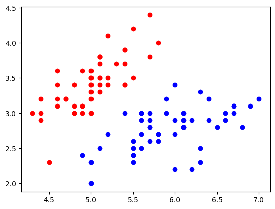
接下来在scikit-learn中的鸢尾花iris数据 上试用,考虑到iris数据集一共有四类,而LogisticRegerssion只能解决二分类问题,这里对iris数据集进行一个简单的处理,只保留前两类 ,同时为例方便可视化只取前两列特征 :
1
2
3
4
5
6
7
8
9
10
11
12
13
14
import numpy as npimport matplotlib.pyplot as pltfrom sklearn import datasetsiris = datasets.load_iris() X = iris.data y = iris.target X = X[y<2 , :2 ] y = y[y<2 ] plt.scatter(X[y==0 , 0 ], X[y==0 , 1 ], c='r' ) plt.scatter(X[y==1 , 0 ], X[y==1 , 1 ], c='b' ) plt.show()
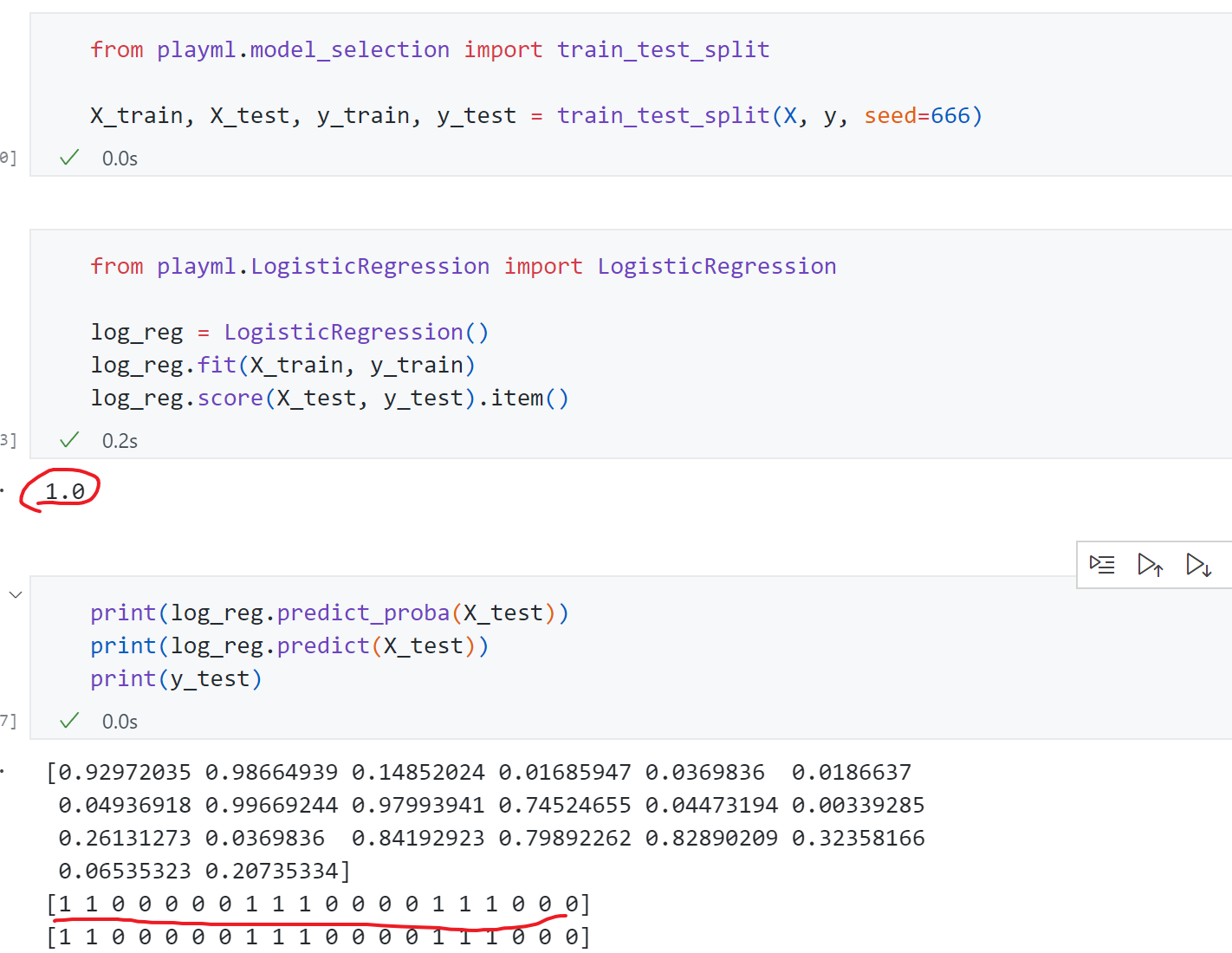
然后训练测试:
测试准确为100%,打印出来可以发先概率以及对应预测的标签,真实标签越接近1的概率越大,真实标签越接近0的概率越小。准确率能100%主要因为iris数据过于简单,同时我们只取了两个特征比较好分类。
决策边界
逻辑回归同样也能求出coef和intercept,那它的几何意义是什么,如何看待这些参数值呢?这就涉及到分类问题一个很重要的概念-决策边界 。
回顾逻辑回归的表达式:
p ^ = σ ( θ T . x b ) = 1 1 + e − θ T . x b y ^ = { 1 , p ^ ≥ 0.5 θ T . x ≥ 0 0 , p ^ ≤ 0.5 θ T . x < 0 \hat{p}=\sigma(\theta^T.x_b)=\frac{1}{1+e^{-\theta^T.x_b}}\\
\hat{y}=
\begin{cases}
1, & \hat{p} \ge 0.5 & \theta^T.x_ \ge0\\
0, & \hat{p} \le 0.5 & \theta^T.x_ <0
\end{cases}
p ^ = σ ( θ T . x b ) = 1 + e − θ T . x b 1 y ^ = { 1 , 0 , p ^ ≥ 0.5 p ^ ≤ 0.5 θ T . x ≥ 0 θ T . x < 0
决策边界为θ T . x b = 0 \theta^T.x_b=0 θ T . x b = 0
如果X有两个特征,则θ 0 + θ 1 x 1 + θ 2 x 2 = 0 \theta_0+\theta_1x_1+\theta_2x_2=0 θ 0 + θ 1 x 1 + θ 2 x 2 = 0
x 2 = − θ 0 − θ 1 x 1 θ 2 x_2=\frac{-\theta_0-\theta_1x_1}{\theta_2}
x 2 = θ 2 − θ 0 − θ 1 x 1
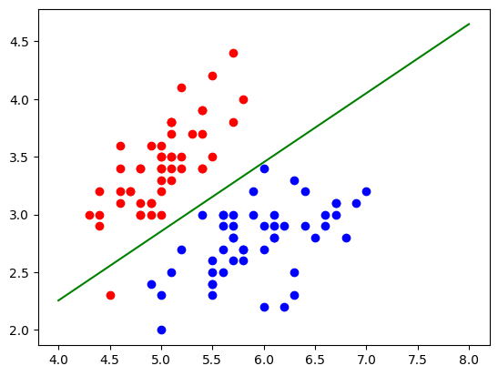
因此绘制一下这个决策边界:
1
2
3
4
5
6
7
8
9
10
def x2 (x1 ): return (-log_reg.coef_[0 ]*x1 - log_reg.interception_ ) / log_reg.coef_[1 ] x1_plot = np.linspace(4 , 8 , 1000 ) x2_plot = x2(x1_plot) plt.scatter(X[y==0 ,0 ], X[y==0 ,1 ], color="red" ) plt.scatter(X[y==1 ,0 ], X[y==1 ,1 ], color="blue" ) plt.plot(x1_plot, x2_plot, c='g' ) plt.show()
绿线即为决策边界 ,>0则分类为1即下方的点,<0上方的点分类为0.同时可以发现 有个红色点分类错误,但是前面测试集准确率100%,说明这个点在训练集中。
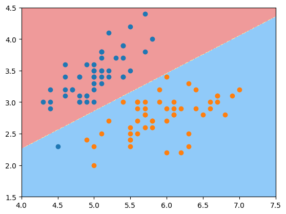
通过上图可以发现,对于逻辑回归算法来说其决策边界是一条直线 ,但其实不论对于KNN,还是逻辑回归,可以加上多项式项使得决策边界不再是一条直线 ,此时需要一种不规则决策边界的绘制方法 。
可以把特征平面看成无数的点,对每一个点都用模型来将其分类,这个过程以此类推对足够密的点继续分类并将颜色绘制出来,就得到了不规则的决策边界。
示例:
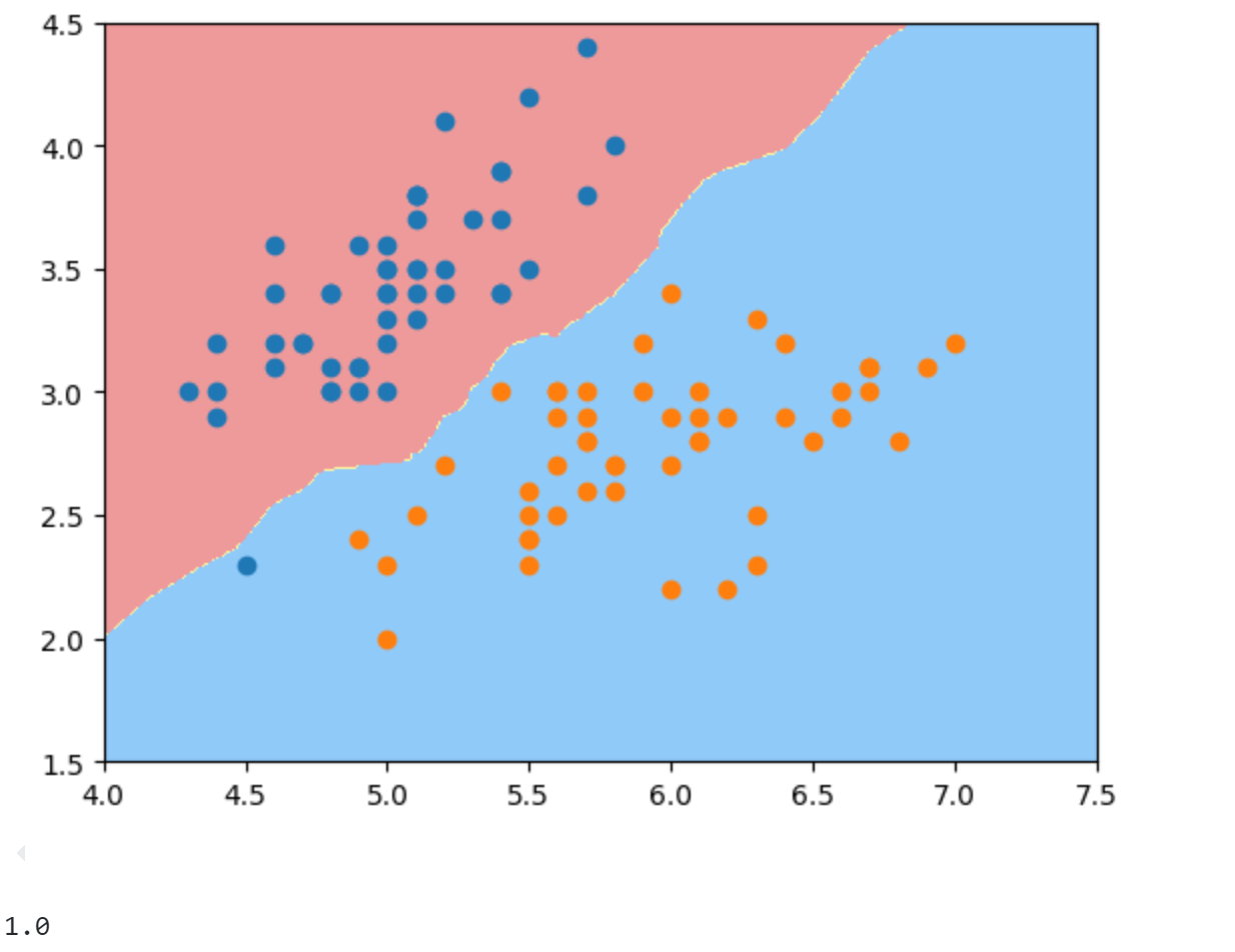
1
2
3
4
5
6
7
8
9
10
11
12
13
14
15
16
17
18
19
20
def plot_decision_boundary (model, axis ): x0, x1 = np.meshgrid( np.linspace(axis[0 ], axis[1 ], int ((axis[1 ]-axis[0 ])*100 )).reshape(-1 , 1 ), np.linspace(axis[2 ], axis[3 ], int ((axis[3 ]-axis[2 ])*100 )).reshape(-1 , 1 ), ) X_new = np.c_[x0.ravel(), x1.ravel()] y_predict = model.predict(X_new) zz = y_predict.reshape(x0.shape) from matplotlib.colors import ListedColormap custom_cmap = ListedColormap(['#EF9A9A' ,'#FFF59D' ,'#90CAF9' ]) plt.contourf(x0, x1, zz, linewidth=5 , cmap=custom_cmap) plot_decision_boundary(log_reg, axis=[4 , 7.5 , 1.5 , 4.5 ]) plt.scatter(X[y==0 ,0 ], X[y==0 ,1 ]) plt.scatter(X[y==1 ,0 ], X[y==1 ,1 ]) plt.show()
同理看一下KNN算法的决策边界,虽然KNN不像逻辑回归有决策边界的表达式,但依然可以通过上面提到的方式绘制出来:
1
2
3
4
5
6
7
8
9
10
from sklearn.neighbors import KNeighborsClassifierknn_clf = KNeighborsClassifier() knn_clf.fit(X_train, y_train) print (knn_clf.score(X_test, y_test))plot_decision_boundary(knn_clf, axis=[4 , 7.5 , 1.5 , 4.5 ]) plt.scatter(X[y==0 ,0 ], X[y==0 ,1 ]) plt.scatter(X[y==1 ,0 ], X[y==1 ,1 ]) plt.show()
可以发现KNN分类准确率也为100%,边界画出来是一条弯曲的曲线。
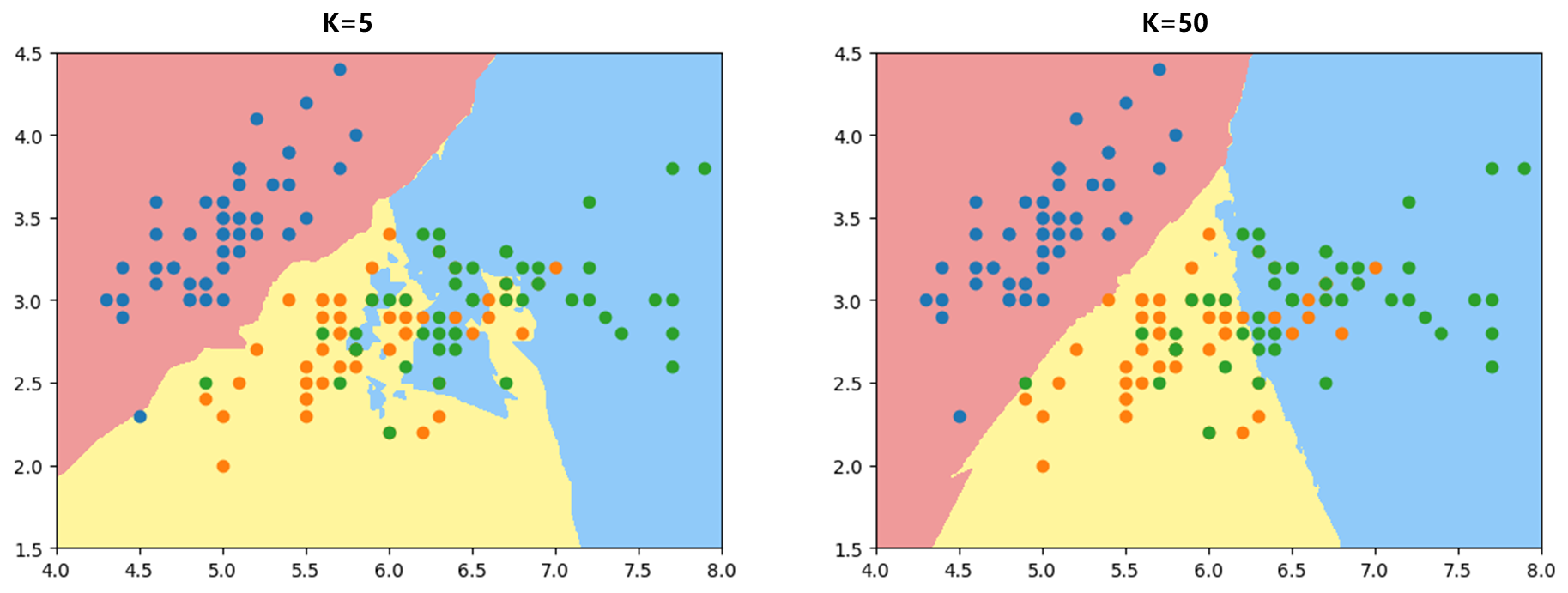
因为KNN可以解决多分类问题,所以尝试对iris三个类别进行分类可视化:
1
2
3
4
5
6
7
knn_clf_all = KNeighborsClassifier() knn_clf_all.fit(iris.data[:,:2 ], iris.target) plot_decision_boundary(knn_clf_all, axis=[4 , 8 , 1.5 , 4.5 ]) plt.scatter(iris.data[iris.target==0 ,0 ], iris.data[iris.target==0 ,1 ]) plt.scatter(iris.data[iris.target==1 ,0 ], iris.data[iris.target==1 ,1 ]) plt.scatter(iris.data[iris.target==2 ,0 ], iris.data[iris.target==2 ,1 ])
可以发现k = 5 k=5 k = 5 k = 50 k=50 k = 50
多项式特征的逻辑回归
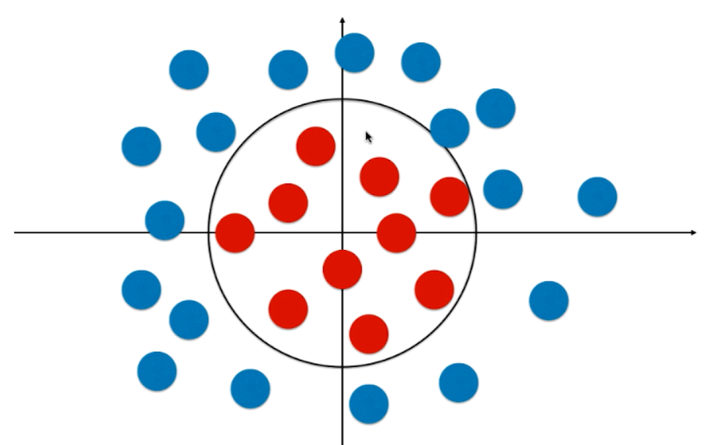
逻辑回归本质上在特征平面中找到一条直线分割样本两个分类,因此只可以解决二分类问题。但是实际问题中决策边界是大概率不规则的比如下面的圆形:
此时要找的边界应满足圆的方程: x 1 2 + x 2 2 = r 2 x_1^2+x_2^2=r^2 x 1 2 + x 2 2 = r 2 引入多项式项 即可。
通过多项式的组合构建几乎可以得到任意形状的决策边界。
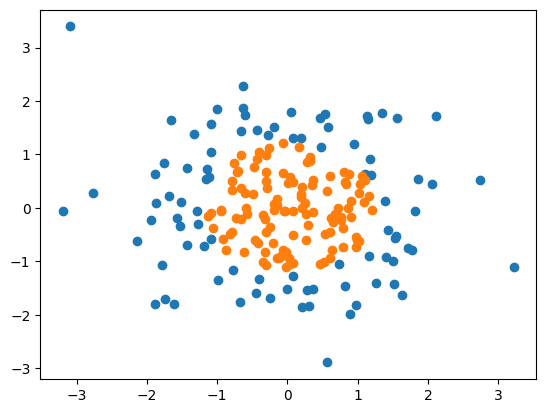
编程示例:
1
2
3
4
5
6
7
8
9
10
import numpy as npimport matplotlib.pyplot as pltnp.random.seed(666 ) X = np.random.normal(0 , 1 , size=(200 ,2 )) y = np.array(X[:,0 ]**2 + X[:,1 ]**2 <1.5 ,dtype='int' ) plt.scatter(X[y==0 ,0 ],X[y==0 ,1 ]) plt.scatter(X[y==1 ,0 ],X[y==1 ,1 ]) plt.show()
首先使用不加多项式特征的逻辑回归(代码同上面,只是数据改下)
准确率只有60.5%,可以发现决策边界是一条直线,有许多错误分类。
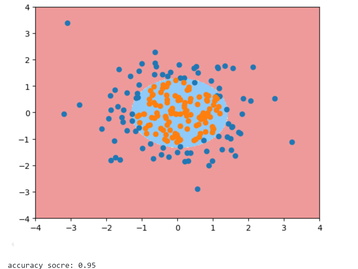
1
2
3
4
5
6
7
8
9
10
11
12
13
14
15
16
17
18
from sklearn.preprocessing import PolynomialFeaturesfrom sklearn.pipeline import Pipelinefrom sklearn.preprocessing import StandardScalerdef PolynomialLogisticRegression (degree ): return Pipeline([ ('poly' , PolynomialFeatures(degree=degree)), ('std_scaler' , StandardScaler()), ('log_reg' , LogisticRegression()) ]) poly_log_reg = PolynomialLogisticRegression(degree=2 ) poly_log_reg.fit(X, y) print ("accuracy socre:" ,poly_log_reg.score(X, y))plot_decision_boundary(poly_log_reg, axis=[-4 , 4 , -4 , 4 ]) plt.scatter(X[y==0 ,0 ], X[y==0 ,1 ]) plt.scatter(X[y==1 ,0 ], X[y==1 ,1 ]) plt.show()
此时准确率有95%,可以发现决策边界是一个圆形,对两类数据进行了很好的划分。
同时注意这里传入的LogisticRegression() 是前面自己定义的类,而不是skleran实现的,但仍能传进去,说明只要遵循sklearn的标注,有fit,predict,score等可以进行无缝衔接。
正则化
逻辑回归既然也可以添加多项式项来生成不规则的决策边界进而对非线性数据进行分类,但引入多项式项模型相应就会变的非常复杂造成过拟合 ,因此为了解决这个问题同样也要正则化 。
前面将多项式回归的正则化方式是给损失函数添加一个L1或L2正则项:
J ( θ ) + α L 1 J ( θ ) + α L 2 J(\theta)+\alpha L_1\\
J(\theta)+\alpha L_2\\
J ( θ ) + α L 1 J ( θ ) + α L 2
Scikit-learn 中的正则化方式 :
C . J ( θ ) + L 1 C . J ( θ ) + L 2 C.J(\theta)+L_1\\
C.J(\theta)+L_2
C . J ( θ ) + L 1 C . J ( θ ) + L 2
超参数C放在了损失函数面前,使用这种方式就不得不正则化,因为L1和L2前面系数至少是1.
scikit-learn中的逻辑回归自动封装了模型正则化项,只需要调整超参数C和正则化方式即可。
因此接下来看下Scikit-learn中的逻辑回归 :
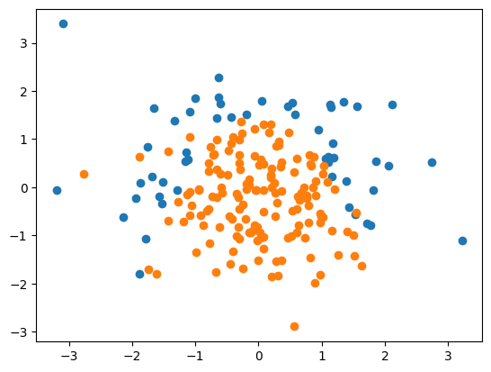
1
2
3
4
5
6
7
8
9
10
11
12
import numpy as npimport matplotlib.pyplot as pltnp.random.seed(666 ) X = np.random.normal(0 , 1 , size=(200 , 2 )) y = np.array((X[:,0 ]**2 +X[:,1 ])<1.5 , dtype='int' ) for _ in range (20 ): y[np.random.randint(200 )] = 1 plt.scatter(X[y==0 ,0 ], X[y==0 ,1 ]) plt.scatter(X[y==1 ,0 ], X[y==1 ,1 ]) plt.show()
要注意一下这里构造y时使用的是抛物线(x 0 2 + x 1 x_0^2+x_1 x 0 2 + x 1
1
2
3
y = np.array((X[:,0 ]**2 +X[:,1 ])<1.5 , dtype='int' ) for _ in range (20 ): y[np.random.randint(200 )] = 1
因为牵扯到正则化,所以上面代码里随机选取了20个点强制其标签为1来添加噪声。
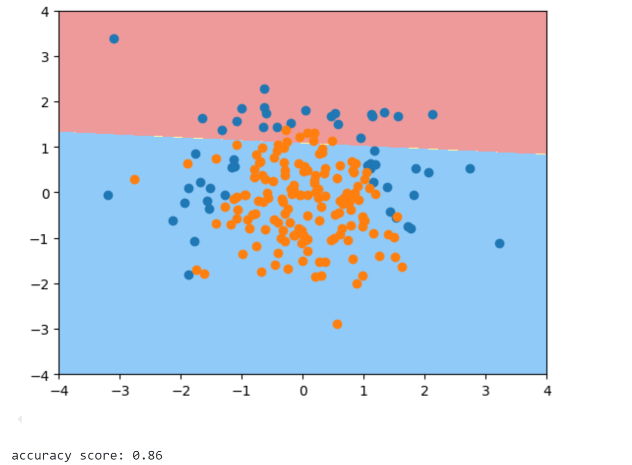
1
2
3
4
5
6
7
8
9
10
11
12
13
14
15
16
17
18
19
20
21
22
23
24
25
26
27
28
29
30
from sklearn.model_selection import train_test_splitX_train, X_test, y_train, y_test = train_test_split(X, y, random_state=666 ) from sklearn.linear_model import LogisticRegressionlog_reg = LogisticRegression() log_reg.fit(X_train, y_train) def plot_decision_boundary (model, axis ): x0, x1 = np.meshgrid( np.linspace(axis[0 ], axis[1 ], int ((axis[1 ]-axis[0 ])*100 )).reshape(-1 , 1 ), np.linspace(axis[2 ], axis[3 ], int ((axis[3 ]-axis[2 ])*100 )).reshape(-1 , 1 ), ) X_new = np.c_[x0.ravel(), x1.ravel()] y_predict = model.predict(X_new) zz = y_predict.reshape(x0.shape) from matplotlib.colors import ListedColormap custom_cmap = ListedColormap(['#EF9A9A' ,'#FFF59D' ,'#90CAF9' ]) plt.contourf(x0, x1, zz, linewidth=5 , cmap=custom_cmap) plot_decision_boundary(log_reg, axis=[-4 , 4 , -4 , 4 ]) plt.scatter(X[y==0 ,0 ], X[y==0 ,1 ]) plt.scatter(X[y==1 ,0 ], X[y==1 ,1 ]) plt.show() print ("accuracy score:" ,log_reg.score(X_test, y_test))
测试集准确率为86%,同时可以发现决策边界是一条直线。
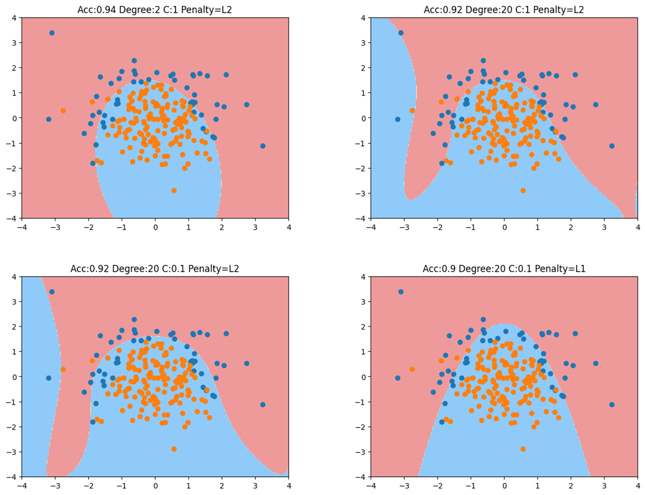
1
2
3
4
5
6
7
8
9
10
11
12
13
14
15
16
17
18
19
20
from sklearn.pipeline import Pipelinefrom sklearn.preprocessing import PolynomialFeaturesfrom sklearn.preprocessing import StandardScalerdef PolynomialLogisticRegression (degree, C, penalty='l2' ): return Pipeline([ ('poly' , PolynomialFeatures(degree=degree)), ('std_scaler' , StandardScaler()), ('log_reg' , LogisticRegression(C=C, penalty=penalty,solver='liblinear' )) ]) poly_log_reg = PolynomialLogisticRegression(degree=20 , C=0.1 , penalty='l2' ) poly_log_reg.fit(X_train, y_train) plot_decision_boundary(poly_log_reg, axis=[-4 , 4 , -4 , 4 ]) plt.scatter(X[y==0 ,0 ], X[y==0 ,1 ]) plt.scatter(X[y==1 ,0 ], X[y==1 ,1 ]) plt.title(f"Acc:{poly_log_reg.score(X_test, y_test)} Degree:20 C:0.1 Penalty=L1" ) plt.show()
d e g r e e = 2 , C = 1 degree=2,C=1 d e g ree = 2 , C = 1
d e g r e e = 20 , C = 1 degree=20,C=1 d e g ree = 20 , C = 1
d e g r e e = 20 , C = 0.1 degree=20,C=0.1 d e g ree = 20 , C = 0.1
d e g r e e = 20 , C = 0.1 , L 1 正则 degree=20,C=0.1,L1正则 d e g ree = 20 , C = 0.1 , L 1 正则 d e g r e e = 20 degree=20 d e g ree = 20
OvR与OvO
逻辑回归只能解决二分类问题,如何改造才能解决多分类问题呢?一般改造方式有两种OvR和OvO ,这两种改造方式对几乎所有二分类算法都适用。
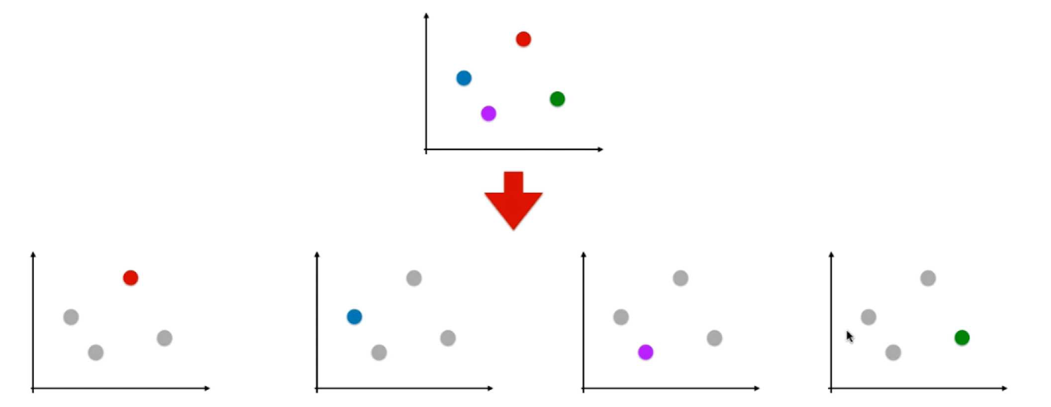
OvR即One vs Rest :
如上图假设有四个类别,我们将红色类别看为一类,剩下的蓝紫绿看为其他类别,此时四分类问题就转变为了二分类问题,此时就可以使用逻辑回归算法。同理就可以一共形成四个分类问题,每一个都是一种颜色和其余颜色的和进行分类。如果有n个类别就进行n次分类,选择分类得分最高的。缺点就是时间复杂度变高了。
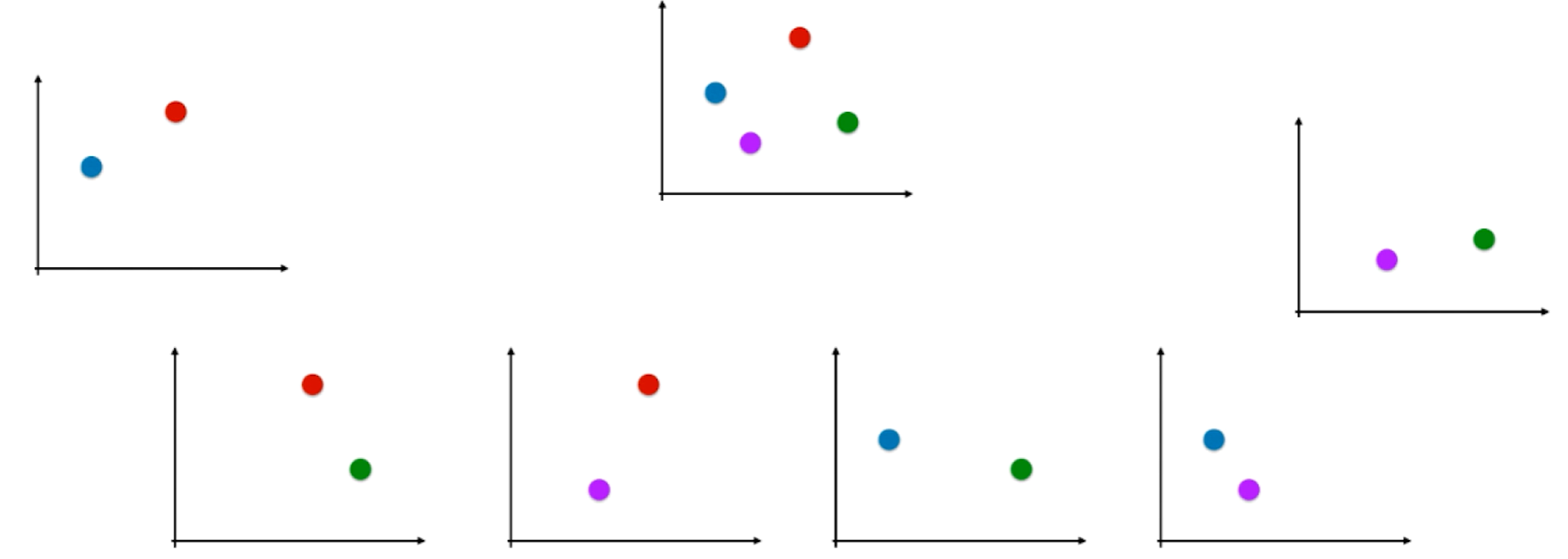
OvR即One vs One :
如上图每次只针对两个类别进行分类,一共有C 4 2 = 6 C_4^2=6 C 4 2 = 6 C n 2 C_n^2 C n 2
显然OVO的方式的时间复杂度是n 2 n^2 n 2
以iris鸢尾花数据集进行示例:
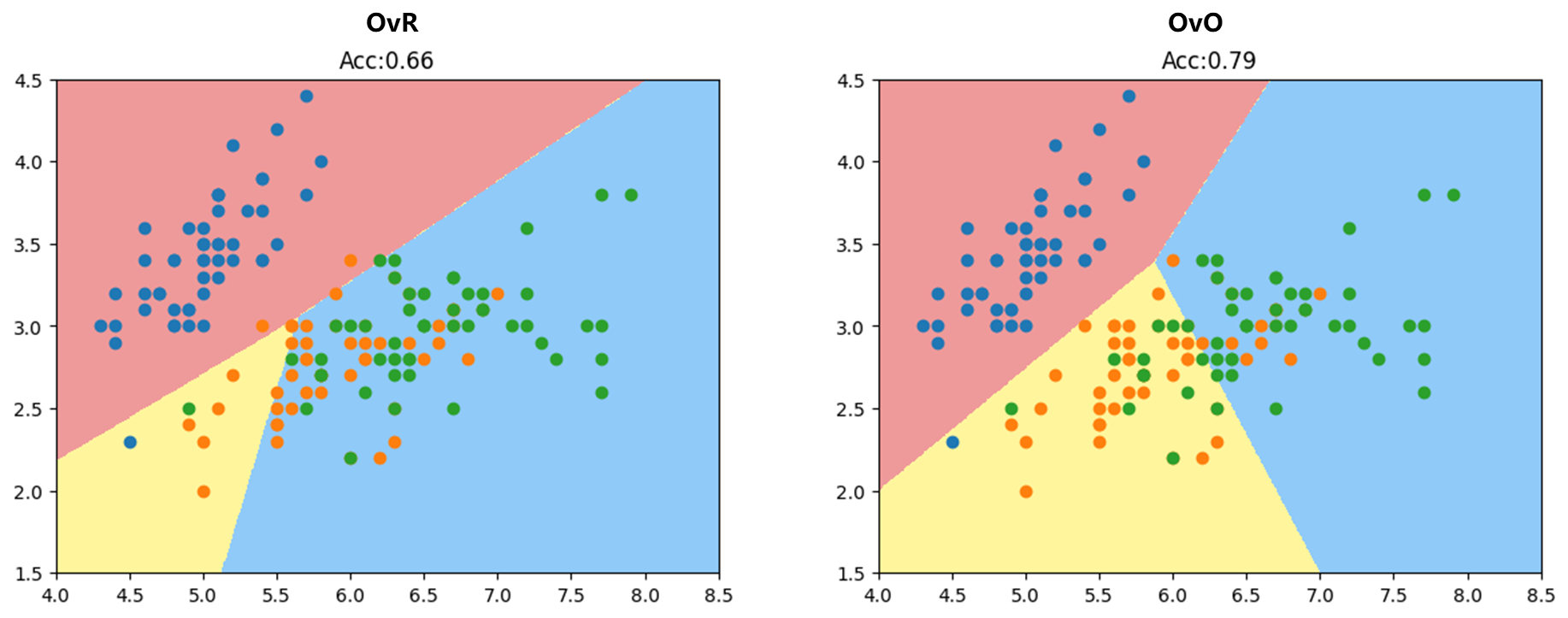
OvR方式和OvO 方式(为了便于可视化先只用到数据的前2个特征)
1
2
3
4
5
6
7
8
9
10
11
12
13
14
15
16
17
18
19
20
21
22
23
24
25
26
27
28
29
30
31
32
33
34
35
36
37
38
39
import numpy as npimport matplotlib.pyplot as pltfrom sklearn import datasetsiris = datasets.load_iris() X = iris.data[:,:2 ] y = iris.target from sklearn.model_selection import train_test_splitX_train, X_test, y_train, y_test = train_test_split(X, y, random_state=666 ) from sklearn.linear_model import LogisticRegressionlog_reg = LogisticRegression(multi_class="ovr" ) log_reg.fit(X_train, y_train) def plot_decision_boundary (model, axis ): x0, x1 = np.meshgrid( np.linspace(axis[0 ], axis[1 ], int ((axis[1 ]-axis[0 ])*100 )).reshape(-1 , 1 ), np.linspace(axis[2 ], axis[3 ], int ((axis[3 ]-axis[2 ])*100 )).reshape(-1 , 1 ), ) X_new = np.c_[x0.ravel(), x1.ravel()] y_predict = model.predict(X_new) zz = y_predict.reshape(x0.shape) from matplotlib.colors import ListedColormap custom_cmap = ListedColormap(['#EF9A9A' ,'#FFF59D' ,'#90CAF9' ]) plt.contourf(x0, x1, zz, linewidth=5 , cmap=custom_cmap) plot_decision_boundary(log_reg, axis=[4 , 8.5 , 1.5 , 4.5 ]) plt.scatter(X[y==0 ,0 ], X[y==0 ,1 ]) plt.scatter(X[y==1 ,0 ], X[y==1 ,1 ]) plt.scatter(X[y==2 ,0 ], X[y==2 ,1 ]) plt.title(f"Acc:{log_reg.score(X_test, y_test):.2 f} " ) plt.show()
可以见OvO方式分类结果更加准确。
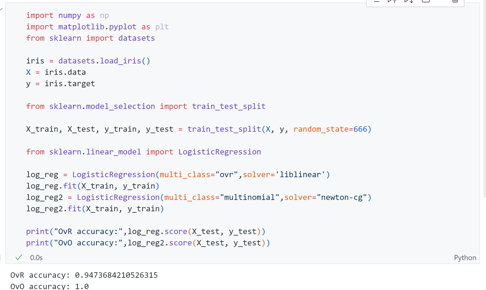
上面是为了可视化方便了只用到了iris的前两个特征,接下来看一下使用所有的特征时模型分类准确度:
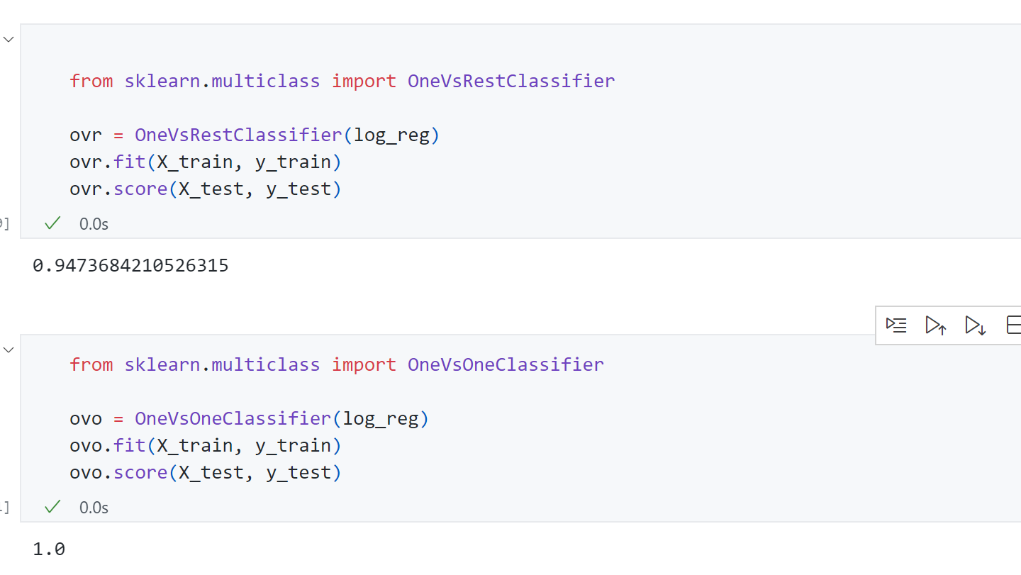
可见使用上所有特征后OvR准确率为94%,而OvO为100%。
同时Scikit-learn还封装了两个类来支持OvR和OvO功能:
传入参数是一个二分类器比如LogisticRegression.